Add a new page:
Add a new page:
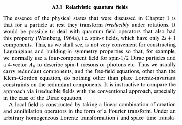
Equations of Motion
The most important equation on modern physics are equations of motions. These equations tell us how a system will evolve as time passes on. We can derive these equations using symmetry considerations from the corresponding Lagrangian using the Euler-Lagrange Equations.
| Important in: | Relationship: | Used For: | ||
| Schrödinger Equation | Quantum Mechanics, Quantum Field Theory | non-relativistic limit of the Klein-Gordon Equation | Describes time evolution | linear |
| Klein-Gordon Equation | Quantum Field Theory | Equation of motion for particles with spin 0 | linear | |
| Pauli Equation | Quantum Mechanics | non-relativistic limit of the Dirac Equation | Equation of motion for particles with spin 1/2 | linear |
| Dirac Equation | Quantum Field Theory | Equation of motion for particles with spin 1/2 | linear | |
| Maxwell Equations | Classical Electrodynamics, Quantum Field Theory | special case of the Yang-Mills equation for a non-abelian gauge theory | Equation of motion for particles with spin 1 in abelian gauge theories | linear |
| Einstein Equation | General Relativity | Describes how spacetime gets curved through energy and matter | non-linear | |
| Yang-Mills Equation | Quantum Field Theory | Equation of motion for particles with spin 1 in non-abelian gauge theories | non-linear | |
| The Navier-Stokes Equations | Hydrodynamics | Describe the flow of fluids | non-linear |
Supplementary equations and boundary conditions
| Equation of Motion | ||||||
| System specific additions, like the interactions/forces acting on the object in question | ||||||
| Boundary conditions | ||||||
| Solutions | ||||||
The equations of motion are usually not enough to describe a system. Especially in the Newtonian framework, we need additional equations that give us, for example, the correct formulas which describe a force that acts on the object in question. For example,
In addition, we always need to specify the Boundary Conditions for the system in question.
Unfortunately, knowing how to write down the equations is not the same as being able to solve them. For example, we know very well the equations of motions describing how a river flows. But as soon as it flows quickly over rough grounds, such that it becomes turbulent, we are no longer able to solve the equations. In such cases we are often forced to revert to the simulation methods discussed previously. […] Thus, only for very, very simple theories it is possible to solve these equations exactly. For theories like the standard model, one has to introduce severe approximations (often called truncations) to be able to solve them. If these approximations are made wisely and with insight, these approximations are such that still questions we have to the theory can be answered correctly. But it takes often very long to understand how to do approximations right.
http://axelmaas.blogspot.de/2012/03/equations-that-describe-world.html
Linear vs. Non-Linear Equations
An important distinction is between linear and non-linear equations. It depends on whether an equation is linear or non-linear in what kind of solutions we are interested in:
Solitons are solitary waves that preserve their speeds and shapes after mutual collision. They play a role in the construction of complete solutions for the nonlinear wave equation that corresponds to the role played by Fourier components in the construction of solutions for linear wave equations.
http://garfield.library.upenn.edu/classics1979/A1979HF81700001.pdf
We consider first the sourceless equation in four dimensions,
$$ D_\mu F^{\mu\nu} = 0. \tag{2.65}$$
[…]
The first issue concerns the existence of regular solutions. If regular initial data is taken, will the solution evolve in a regular fashion, or will the nonlinearities produce singularities? This question has been answered: regular solutions to (2.65) do exist, and the same is true if one considers a larger system: scalar and spinor fields interacting with gauge fields [20].
However, physicists are not so interested in the general solution which depends on arbitrary initial data, but rather in specific solutions which reflect some physically interesting situation. For example, in the Maxwell theory we are interested in plane wave solutions.
Let us note that any Maxwell solution is a solution of the Yang-Mills equation, when one makes the Ansatz that the space and internal symmetry degrees of freedom decouple. If one forms $A_\mu^a(x) = \eta^a A_\mu (x)$ with $\eta^a$ constant and $A_\mu(x)$ satisfying the Maxwell equation, then $A_\mu^a(x)$ is a solution to the Yang-Mills equation, which we shall call "Abelian. Thus it is interesting the see whether there are plane wave solutions in the non-Abelian theory, which are not Abelian. By "plane wave", we shall mean a configuration of finite energy $(0 < \mathcal{e} < \infty$), of constant direction for the Poynting vector $\mathcal{P}(x) = \hat{\mathcal{P}}|\mathcal{P}(x)|$ with $\hat{\mathcal{P}}$ constant, and with magnitude of the Poynting vector equal to the energy density $ \mathcal{e} = \mathcal{P}(x)|$. Such solutions have been constructed [21], but unlike their Maxwell analogs, they do not seem to have any physical significance. certainly, if gauge quanta are confined, one cannot make a coherent superposition of the to construct an observable plane wave. Alternatively, one may view the Maxwell waves as quantum mechanical wave functions for the photon. However, the non-Abelian plane waves solve a nonlinear equation; they cannot be superposed to form other solutions, and it is hard to see how they can be used as wave functions.
Another class of solutions, more appropriate to nonlinear field theories, are the celebrated solitons, which do have a quantum meaning - they are the starting point of a semi-classical description of coherently bound quantum states [22]. A soliton should be a static solution, have finite energy, and be stable in the sense that small perturbations do not grow exponentially in time. However, one proves with virial theorems that no such solution exists in the pure Yang-Mills theory in four, three or two dimensions [23].
Another tack that one take is that of symmetry. Recall that the classical Yang-.Mills theory in four dimensions possesses conformal $SO(4,2)$ symmetry. One may seek solutions invariant under the maximal compact subgroup, i.e. $SO(4) \times SO(2)$. This solution has been constructed [24]; it is called a "meron". But again no physical significance has been attached to it, or to its generalization which possesses the smaller compact invariance symmetry group $SO(4)$ [25].
There are many other solutions to (2.65) that have been found [26], and while their discoverers invariably highlight some unique characteristic, no physical application has been given thus far - although doubtlessly they are mathematically interesting.
[…]
There is one more class of solutions, which I shall describe later. These do not solve the Yang-Mills equations (2.65) in Minkowski space, but rather in Euclidean space, and are called instantons (pseudoparticles). In fact instantons solve the self-duality equation
$$ ^\star F^{\mu\nu} = \pm F^{\mu\nu} $$
and then (the Euclidean-space analog of) (2.65) follows by the Bianchi identity. […] Of all the solutions, the instantons have interested mathematicians most; for physicists they give a semi-classical understanding of some of the topological effects that are present in Yang-Mills theory.
Topological Investigations of Quantized Gauge Theories, by R. Jackiw (1983)
Moreover, it's important whether the equation contains spinors or scalars and vectors. If there are spinors in the equation we can't construct macroscopic solutions. The reason for this is the Pauli principle that forbids that particles describe by spinors occupy the same state.
[V]ia the Pauli exclusion principle, fermions cannot occupy the same state within the same macro system. So, whereas photons (bosons) can occupy the same state and a lot of them can therefore reinforce one another to produce a macroscopic electromagnetic field, spinors (fermions) cannot do so. In other words, we have no classical macroscopic spinor fields to sense, interact with, and study experimentally. And thus, we have no classical theory of spinors.
Student Friendly Quantum Field Theory by Klauber
In addition, it is important to note that the solutions of, for example, the Maxwell equations can be interpreted to describe a single photon or also the whole electromagnetic field.
Similarly, solutions of the Dirac equation can be interpreted to describe a single electron or the whole electron field.
Like the Hamiltonian formalism for classical physics, the Schrödinger equation is not so much a specific equation, but a framework for quantum mechanical equations generally. Once one has obtained the appropriate Hamiltonian, the time evolution of the state according to Schrödinger's equation proceeds rather as though $|\Psi>$ were a classical field subject to some classical field equation such as Maxwell's. In fact, if $|\Psi>$ describes the state of a single photon, then it turns out that Schrodinger's equation actually becomes Maxwell's equations! The equation for a single photon is precisely the same as the equation for an entire electromagnetic field. (However, there is an important difference in the type of solution for the equations that is allowed. Classical Maxwell fields are necessarily real whereas photon states are complex. There is also a so-called 'positive frequency condition that the photon state must satisfy). This fact is responsible for the Maxwell-field-wavelike behaviour and polarization of single photons that we caught glimpses of earlier. As another example, if 11Ji} describes the state of a single electron, then Schröinger's equation becomes Dirac's remarkable wave equation for the electron discovered in 1928 after Dirac had supplied much additional originality and insight
The Emperor's New Mind by R. Penrose
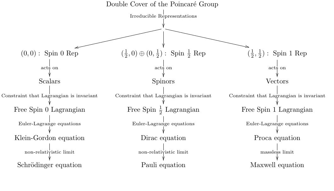
One popular way to derive the fundamental equations of nature is to use the Lagrangian formalism.
This procedure is demonstrated explicitly, for example, in the book "Physics from Symmetry" by J. Schwichtenberg.
A broad outline of the derivation looks as follows:
Most of the fundamental equations can be used either in a particle theory or in a field theory. In a particle theory, the solutions describe particle trajectories:
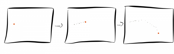
while in a field theory the solutions describe sequences of field configurations:

For a nice discussion, see The equations that describe the world by Axel Maas.
The Equations of Motion yield the Most Important Paths
In the path integral formuation of quantum mechanics, particles do not follow one individual path but instead all of them. Hence there can't be one equation whose solution yields the correct particle trajectory.
However, the equations of motion are still important and the path integral formalism tells us why.
While we must consider all possible paths, the most important path is still the path that we get by solving the equation of motion. In the path integral formalism, all paths are weighted by their corresponding action. The equations of motion are derived by extremizing the action. Hence, the biggest contribution to the whole path integral comes from those paths with extremal action, which are precisely those that we get by solving the equations of motion.
Formulated differently, the thing is that a particle really has some probability to go all possible ways. However, the classical path is the most probable path, because paths close this path infer constructively and hence yield a big probability. In contrast, for other paths far away from the classical path the interference is destructive and hence the probability is tiny. The path with minimal action gives the biggest contribution to the path integral in the classical limit $\hbar \to 0$.
This is explained nicely in Section 3 here.
Take note that the interpretation also works for field theories. However, in field theory we, of course, do not consider particle paths but sequences of field configurations. The solutions of the field equation then describe the most probably sequence of field configurations.
The Equations of Motion are Constraint Equations
A massless spin 1 particle has 2 degrees of freedom. However, we usually describe it using four-vectors, which have four components. Hence, somehow we must get rid of the superfluous degrees of freedom. This job is done by the Maxwell equations.
“In some sense, Maxwell's equations were a historical accident. Had the discovery of quantum mechanics preceded the unification of electricity and magnetism, Maxwell's equations might not have loomed so large in the history physics. … Since the quantum description has only two independent components associated with each four momentum, there are four dimensions worth of linear combinations of the classical field components that do not describe physically allowed states, for each four momentum. Some mechanism must be derived for annihilating these superpositions. This mechanism is the set of equations discovered by Maxwell. In this sense, Maxwell's equations are an expression of our ignorance.”Gilmore's "Lie Groups, Physics, and Geometry"
Fields in physics are something which associate with each point in space and with each instance in time a quantity. In case of electromagnetism this is a quantity describing the electric and magnetic properties at this point. Each of these two properties turn out to have a strength and a direction. Thus the electric and magnetic fields associate with each point in space and time an electric and a magnetic magnitude and a direction. For a magnetic field this is well known from daily experience. Go around with a compass. As you move, the magnetic needle will arrange itself in response to the geomagnetic field. Thus, this demonstrates that there is a direction involved with magnetism. That there is also a strength involved you can see when moving two magnets closer and closer together. How much they pull at each other depends on where they are relative to each other. Thus there is also a magnitude associated with each point. The same actually applies to electric fields, but this is not as directly testable with common elements. Ok, so it is now clear that electric and magnetic fields have a direction and a magnitude. Thus, at each point in space and time six numbers are needed to describe them: two magnitudes and two angles each to determine a direction.
When in the 19th century people tried to understand how electromagnetism works they also figured this out. However, they made also another intriguing discovery. When writing down the laws which govern electromagnetism, it turns out that electric and magnetic fields are intimately linked, and that they are just two sides of the same coin. That is the reason to call it electromagnetism.
In the early 20th century it then became clear that both phenomena can be associated with a single particle, the photon. But then it was found that to characterize a photon only two numbers at each point in space and time are necessary. This implies that between the six numbers characterizing electric and magnetic fields relations exist. These are known as Maxwell equations in classical physics, or as quantum Maxwell dynamics in the quantum theory. If you would add, e. g., electrons to this theory, you would end up with quantum electro dynamics - QED. http://axelmaas.blogspot.de/2010/10/electromagnetism-photons-and-symmetry.html
Analogously, we can interpret the other equations of motion. For the Dirac equation, this is discussed nicely at page 444ff in the book "Spin in Particle Physics" by Elliot Leader: