Canonical Quantum Field Theory

Intuitive

The basic object is the ocean. In the context of particle physics, this ocean is then called a field. Such a field is now existing at every point in space and at every instance in time. In the very literally meaning of the word, it fills up all of the universe. If there is nothing of interest around, this is because the size of the field at this point in space and time is small or even vanishing. However, if there is a spike at some point in the field then just as in the picture of the ocean there sits a particle. If there is a second spike somewhere else, then there is another particle, and so on. Since all the spikes belong to the same field, they describe the same type of particle, say an electron. The spikes may move with different speeds, so the electrons appear to have different speeds, but they are still electrons. That is the reason why all electrons are the same: They are just spikes in the same field. Such a spike is often called an excitation of the field, and this excitation is the electron.

Then what is about the other types of particles? The quarks, the gluons, the Higgs? Well, these belong just to other fields. That is, our universe is filled up with many fields, all existing simultaneously at every point in space and time.

You may be wondering how this should work, and if this is not a bit crowded. But you know already that fields are mathematical concepts. For example, you can associate with every point in space and time a temperature, and thus create a temperature field. At the same time, there is an atmospheric pressure field. Both can happily exist simultaneously. But they are not ignoring each other. As you know, both are related with each other: If either changes this indicates a change of the other as well. Though this analogy is not exactly the same as the particle physics fields, and there are more things involved, the basic idea is the same.

Also the particle physics fields interact, and thus not ignore each other. […]

We are then 'just' a very complicated, combined, and correlated simultaneous excitation of all of these fields, as is your desk or your computer.

http://axelmaas.blogspot.de/2012/01/wave-functions-and-fields-once-more.html

Quantum fields are not mysterious after all. For a nice explanation of how to think about them have a look at A Children’s Picture-book Introduction to Quantum Field Theory by Brian Skinner. Further explanations, from the same author can be found here, here and here. (The math behind this description can be found, for example in "QFT in a Nutshell" by A. Zee or chapter 1 here.)

For another article series in the same spirit see this series by Matt Strassler.
“Our stability is but balance” — Freeman Dyson on how to imagine quantum fields
“So is the universe made of tiny springs, or isn’t it?” by Brian Skinner
A nice book that explains many of the most important concepts of QFT in Laymen terms is "A Zeptospace Odyssey: A Journey Into the Physics of the LHC" by Gian Francesco Giudice
Another book, with a historical perspective and many nice stories and explanations is "The Infinity Puzzle" by F. Close
The most famous laymen QFT book is "QED: The Strange Theory of Light and Matter" by Richard P. Feynman
Another nice intro is the series by Flip Tanedo.

Concrete

Before reading anything else, you should read the "Bird’s Eye View" of quantum field theory by Robert Klauber.

Arguably the most important equation of quantum field theory is the canonical commutation relation \begin{equation} \label{qftcomm} [\Phi(x), \pi(y)]=\Phi(x) \pi(y) - \pi(y) \Phi(x) = i \delta(x-y) \end{equation} where $\delta(x-y)$ is the Dirac delta distribution and $\pi(y) = \frac{\partial \mathscr{L}}{\partial(\partial_0\Phi)}$ is the conjugate momentum.

This canonical commutation relation is often stated as a postulate, which marks the starting point of quantum field theory.

It tells us that the fields in quantum field theory $\Phi(x)$ can‘t be simply a function, but must be operators. Ordinary functions and numbers commute:

For example $f(x)=3x$ and $g(y)= 7y^2 +3$ clearly commute $$ [f(x) , g(x)]= f(x)g(x) - g(x) f(x) = 3x (7y^2 +3) -(7y^2 +3) 3x =0. $$

Therefore, we have to conclude that quantum fields are operators that act, like every operator in quantum theory, on abstract states.

To understand the fields a bit better we look at a concrete example.

Example: A Scalar Field

A free spin $0$ field (= a scalar field) obeys the Klein-Gordon equation. The general solution of this equation can be written as

\begin{equation}\label{KGsol} \Phi(x)= \int \mathrm{d }k^3 \frac{1}{(2\pi)^3 2\omega_k} \left( a(k){\mathrm{e }}^{ -i(k x)} + a^\dagger(k) {\mathrm{e }}^{ i(kx)}\right)\end{equation}

Now, if we combine this solution with the canonical commutation relation we see that $a(k)$ and $a^\dagger(k)$ can‘t be numbers, but must be operators. Using $[\Phi(x), \pi(y)] = i \delta(x-y)$ we can compute

$$ [a^\dagger(k), a(k)] = i \delta(x-y) .$$

Everything else in the solution are just ordinary numbers.

So what are these operators?

To answer this question, we next look at something that we understand: energy.

Using the Lagrangian, we can compute the corresponding Hamiltonian, which represents the energy and is the conserved quantity that follows from invariance under time-translation, according to Noether‘s theorem.

For example, for spin $0$ fields we have\begin{equation} \label{hamil} H= \frac{1}{2} \Big( \big(\partial_0 \Phi \big)^2 + ( \partial_i \Phi )^2 + m \Phi^2 \Big). \end{equation}The fields are operators and therefore the Hamiltonian is an operator. For reasons explained above we call it the energy operator, which means if we act with the Hamiltonian on an abstract state $ | \Psi \rangle$ that describes the system in question, we get the energy of the system:$$ H | \Psi \rangle = E | \Psi \rangle $$

Do the operators $a(k)$ and $a^\dagger(k)$ have any effect on the energy of the system? That may seem like a strange question, but will make a lot of sense in a moment. To find an answer we must compute $H a(k) | \Psi \rangle$.

Click here to see some details how we can compute this

This can be done by putting our general solution of the Klein-Gordon equation into the explicit form of the Hamiltonian. This yields $$\hat H =\int \mathrm{d }k^3 \frac{1}{(2\pi)^3 } \omega_k \left(a^\dagger(k) a(k) \right) $$Then we can use Eq. \ref{qftcomm} to compute

\begin{equation}\label{commHunda} [\hat H,a(k')] = - \omega_{k'}a(k') .\end{equation}

We can then compute that

\begin{align} \label{eq:energyloweringdemo} \hat H \left( a(k') | \Psi \rangle \right) &= \left( a(k') \hat H +\underbrace{ \hat H a(k') -a(k') \hat H }_{[ \hat H , a(k')]}\right) | \Psi \rangle \notag \\ &= a(k')\underbrace{ \hat H | \Psi \rangle}_{=E | \Psi \rangle} + [ \hat H , a(k')] | \Psi \rangle \notag \\ &= \Big( a(k') E + [ \hat H , a(k')] \Big) | \Psi \rangle\notag \\ &= \Big( a(k') E - \omega_{k'} a(k')\Big) | \Psi \rangle \notag \\ &= \Big( E - \omega_{k'} ) \left( a(k') | \Psi \rangle\right) \end{align}

The result is:

$$ \hat H \big( a(k') | \Psi \rangle \big) = \Big( E - \omega_{k'} ) \big( a(k') | \Psi \rangle \big) $$

In words this means that our operator $a(k')$ lowers the energy of the system by the amount $ \omega_{k'} $. Equivalently, we can compute that $a^\dagger(k')$ raises the energy by the amount $ \omega_{k'} $.

Imagine we have a completely empty system, which means energy zero:

$$ H | 0\rangle = 0 | 0\rangle $$

If now our operators $a^\dagger(k')$ acts on this completely empty system it suddenly has energy $ \omega_{k'} $ instead of zero:

$$ H a^\dagger(k') | 0\rangle = \omega_{k'} a^\dagger(k') | 0\rangle $$

Therefore $a^\dagger(k') | 0\rangle$ describes a new system, which isn‘t empty any more. We can act again with $a^\dagger(k')$ on this system, which has then energy $2 \omega_{k'} $:

$$ H a^\dagger(k') a^\dagger(k') | 0\rangle = 2\omega_{k'} a^\dagger(k') a^\dagger(k') | 0\rangle $$

Recall that $a^\dagger(k')$ and $a(k')$ are the operator parts of our quantum fields. Here we learn that quantum fields create and annihilate particles!

$| 0\rangle$ is an empty system

$a^\dagger(k') | 0\rangle$ is a system with one particle, with energy $\omega_{k'} $. Therefore we write $a^\dagger(k') | 0\rangle = | 1_{k‘}\rangle$

$a^\dagger(k') a^\dagger(k') | 0\rangle$ is a system with two particles, with energy $\omega_{k'} $ each. Therefore we write $a^\dagger(k') a^\dagger(k') | 0\rangle= | 2_{k‘}\rangle$.

Of course it is possible to create particles with different energy. For example if we consider $a^\dagger(k'‘)a^\dagger(k') a^\dagger(k') | 0\rangle$, we have a system with two particles with energy $\omega_{k'} $ and one with energy $\omega_{k'‘} $. Therefore $a^\dagger(k'‘) a^\dagger(k') a^\dagger(k') | 0\rangle= | 2_{k‘}, 1_{k‘‘}\rangle$.

It‘s absolutely normal to have now thousands of question popping up in your head. You‘re in good company. For example Richard Feynman:

I remember that when someone had started to teach me about creation and annihilation operators, that this operator creates an electron, I said, "how do you create an electron? It disagrees with the conservation of charge", and in that way, I blocked my mind from learning a very practical scheme of calculation.

You‘ll find very good answers to these questions if you dive deeper into the concepts of quantum field theory. Conservation of charge, for example, is never violated. For the moment, the message to take away is: Quantum fields create and annihilate particles.

Scattering in Quantum Field Theory

Most parts of quantum field theory are about scattering processes. This means we want to use the framework to answer questions like: If we smash an electron and a positron together what are the odds that we detect an outgoing photon in our detectors afterwards.

In mathematical terms, using the usual Dirac notion, we can write this question as $$\langle \gamma(k‘)| \hat S | e_ -(p), e_+(p‘) \rangle= ?$$Here $p$ and $p‘$ denote the momentum of the colliding electron and positron, $k$ the momentum of the outgoing photon and $ \hat S$ is some operator that describes the scattering process.

What should this operator do? We start with some state at an initial point in time and want to calculate the probability to find it at some later time in another state. Therefore, the scattering operator is simply the time-evolution operator that is used in quantum mechanics, too.

Time Evolution The time-evolution in quantum mechanics is described by the Schrödinger equation:\begin{equation} \label{eq:schroedinger} i \partial_t | \Psi (t)\rangle = H | \Psi (t)\rangle, \end{equation}where $H$ denotes the Hamiltonian.

Click here to read some thoughts that make plausible why this equation holds in quantum field theory, too.

he Hamiltonian represents the energy of the system in question. Noether‘s theorem tells us that there is direct connection between time-invariance and the conservation of energy.

In mathematical terms this means that if our Lagrangian is invariant under the action of the generator of time-translations $i \partial_t $, the Energy is conserved.

The conserved quantity we get through Noether‘s theorem is the Hamiltonian. Therefore it shouldn‘t be a big surprise that the Hamiltonian is the crucial ingredient that tells us how our system evolves in time.

As an aside: Maybe you never heard the word generator in this context before, but happily this notion is really intuitive. For a function $f(t)$, we can compute the functions value at a later point in time $f(t+a)$, by using the Taylor series

$$ f(t+a) = f(t) +a \partial_t f(t) \ + a^2 \frac{\partial_t^2 f(t)}{2} \+ \ldots $$

In the smallest possible (infinitesimal) case $a \rightarrow \epsilon$, we can neglect higher order terms $\epsilon^2 \approx 0$ etc. and therefore

$$ f(t+\epsilon) = f(t) +\epsilon \partial_t f(t) . $$

Therefore the basic building block generating a translation to a later point in time is really $\partial_t$.

Unfortunately explaining why we have an extra factor $i$ here would lead us a little too far apart, but in short: We need the extra $i$ to get real instead of imaginary energy values.

We can introduce formally an time-evolution operator that enables us to compute how our state transforms from the initial point in time $t_0$ to a later point in time:$$ S(t-t_0) | \Psi (t_0)\rangle = | \Psi (t)\rangle. $$

This means we simply write down what an operator that we call time-evolution operator must do. For notational brevity, let‘s use $t_0=0$, which is just a matter of choice.

$$ S(t) | \Psi (0)\rangle = | \Psi (t)\rangle. $$

We can put this into our equation which yields

\begin{equation} i \partial_t S(t) | \Psi (0)\rangle = H S(t) | \Psi (0)\rangle. \end{equation}

This equation holds for arbitrary $ | \Psi (0)\rangle$ and therefore

\begin{equation} i \partial_t S(t) = H S(t) \end{equation}

The general solution of this equation is

$$ S(t) = \mathrm{e}^{-i \int H dt},$$

because

\begin{align} & \quad i \partial_t S(t) | \Psi (0)\rangle = H S(t) | \Psi (0)\rangle \\ & \rightarrow i \partial_t \mathrm{e}^{-i \int H dt}| \Psi (0)\rangle = H \mathrm{e}^{-i \int H dt} | \Psi (0)\rangle \\ & \rightarrow H \mathrm{e}^{-i \int H dt}| \Psi (0)\rangle = H \mathrm{e}^{-i \int H dt} | \Psi (0)\rangle \end{align}

We conclude: The mysterious scattering operator isn‘t mysterious at all.

Now we have the scattering operator and all we need to compute $$\langle \gamma(k‘)| \hat S | e_ -(p), e_+(p‘) \rangle$$ is $H$.

As noted above, we can compute the Hamiltonian $H$ from the corresponding Lagrangian and the Lagrangian is what defines our physical theory.

The derivation of the Lagrangian that describe the interactions of particles is done using gauge theory.

This yields one Lagrangian (and therefore one Hamiltonian) for electromagnetic interactions, one for weak and one for strong interactions. For example the Lagrangian, describing electromagnetic interactions is$$ H = \int d^3x \left( g A_\mu \bar \Psi \gamma^\mu \Psi \right) $$Here $A_\mu$ describes a spin $1$ field and $\Psi$ a spin $ \frac{1}{2}$ field.

If we want to consider all interactions at once we need to write these into one big Lagrangian and derive the corresponding Hamiltonian.

How Quantum Field Theory Works

We have now everything at hand to understand what is really going on in quantum field theory. To recapitulate:

We want to compute $\langle \gamma(k‘)| \hat S | e_ -(p), e_+(p‘) \rangle$, where $\hat S$ denotes the scattering operator.
We derived $ S(t) = \mathrm{e}^{-i \int H dt}$.
We have $H = \int d^3x \left( g A_\mu \bar \Psi \gamma^\mu \Psi \right) $.
We know that quantum fields create and annihilate particles.

One key feature of quantum field theory is that we can‘t evaluate $ \mathrm{e}^{-i \int H dt}$ simply at once, but must write the exponential function as a series and evaluate the series term by term. Therefore

\begin{align} \hat{S} &= \underbrace{1}_{S^{(0)}} \underbrace{-i \int dt_1 H(t_1)}_{S^{(1)}} \\ & \quad \underbrace{- \frac{1}{2!} T \Bigg \{ \left( \int dt_1 H(t_1) \right) \left( \in dt_2 H(t_2) \right) \Bigg \}}_{S^{(2)}} + \ldots \end{align}

This is possible because we have coupling constants $g$ in the Hamiltonian. The first term is proportional to $g$, the second to $g^2$, the third to $g^3$.

If the coupling constant is smaller than one, the higher order terms of the series expansion are less expansions and we get a good approximation of the solution of we focus on the first few terms.

Happily for electromagnetic and weak interactions the coupling constant is smaller than one!

The first term $S^{(0)}=1$ changes nothing and is only interesting for computations like $\langle e_ -(k), e_+(k‘) | \hat S | e_ -(p), e_+(p‘) \rangle$. The next term of the series $S^{(1)}$ is more interesting. We now need the explicit form of the Hamiltonian, which we cited above.

$$ S_1 = -i \int dt_1 H(t_1) = -i \int dt \int d^3x \left( g A_\mu \bar \Psi \gamma^\mu \Psi \right) $$

Take note that this Hamiltonian takes only electromagnetic interactions into account. If we want to consider weak-interactions, too we need to use a longer and more complicated Hamiltonian.

For each field, we can use the solution of the equations cited at the beginning. Each solution consists of two terms and therefore this one term of the series is actually eight terms. Happily, the interpretation of these terms is straight-forward.

$\Phi= \Phi^+ \Phi^-$, where $ \Phi^+$ annihilates and $\Phi^-$ creates spin $0$ particles.
$\Psi= \Psi^+ \Psi^-$, where $ \Psi^+$ annihilates and $\Psi^-$ creates spin $\frac{1}{2}$ particles.
$\bar \Psi= \bar \Psi^+\bar \Psi^-$, where $ \bar \Psi^+$ annihilates and $\bar \Psi^-$ creates spin $\frac{1}{2}$ anti-particles.
$A_\mu= A_\mu^+A_\mu^-$, where $ A_\mu^+$ annihilates and $A_\mu^-$ creates spin $1$ particles.

We will focus here on only one of these terms and you‘ll understand in a moment why:

$$ \langle \gamma(k‘)| \hat S | e_ -(p), e_+(p‘) \rangle \approx \langle \gamma(k‘)| ig \int d^4x A_\mu^- \bar \Psi^+ \gamma^\mu \Psi^+|e^-(p), e^+(p‘)\rangle$$

What happens here? Well, $\Psi^+$ destroys the electron, $\bar \Psi^+$ destroys the positron, which leaves us with an empty system:

$$ \langle \gamma(k‘)| ig \int d^4x A_\mu^+ \bar \Psi^+ \gamma^\mu \Psi^+|e^-(p), e^+(p‘)\rangle $$ $$ = \langle \gamma(k‘)| const \times ig \int d^4x A_\mu^- |0 \rangle $$

Then $A_\mu^-$ creates a photon:

$$ \langle \gamma(k‘)| const \times ig \int d^4x A_\mu^- | 0\rangle = \langle \gamma(k‘)| const' \times ig \int d^4x | \gamma(p+p‘) \rangle$$

$ \gamma(p+p‘) \rangle$ and $ \langle \gamma(k‘)| $ fit nicely together

$$ \langle \gamma(k‘)| \gamma(p+p‘) \rangle = \delta(k-(p+p‘)) $$

and therefore we get something non-zero. The resulting number is exactly the probability amplitude we are interested in.

For every other term of the sum we would get zero, because for example:

$$ \langle \gamma(k‘)| ig \int d^4x A_\mu^+ \bar \Psi^+ \gamma^\mu \Psi^-|e^-(p), e^+(p‘)\rangle = \langle \gamma(k‘)| const \times ig \int d^4x |e^-(p), e^-(p‘‘) , \gamma(p‘‘‘)\rangle$$

and we have

$$ \langle \gamma(k‘)| |e^-(p), e^-(p‘‘) , \gamma(p‘‘‘)\rangle =0,$$

because the states are orthogonal. This should be plausible, because assume we have just an electron $ |e^-(p)\rangle$ and we want to know what the probability is to find it as an photon at the same moment in time, without any interaction:

$$ \langle \gamma(p)|| e^-(p)\rangle =0 $$

This must be zero. For example, because of charge conservation.

Further Remarks

Please take note that there are, of course, some very important concepts we haven‘t talked about here like the interaction picture, but you can read about these in the books recommended at the bottom of this page. The interaction picture enables us to use everything we learn about free fields, which means fields without interactions, in an interaction theory. The behaviour of free fields are exactly what is described by the equations like the Klein-Gordon or the Dirac equation above.

Best Textbooks:

Introduction to Elementary Particles by Griffiths gives a nice overview, before you start diving into the subject.
Student Friendly Quantum Field Theory by Klauber; is the best textbook on QFT.
Quantum Field Theory and the Standard Model by Schwartz; is a great book with many in-depth explanations. However, before reading it one should already have good grasp of what QFT is all about and where certain concepts fit into the context. Great as a reference.
Quantum Field Theory in a Nutshell by Zee; is a nice and unconventional book. It focusses, in contrast to most other books, on the path integral formulation, and contains many pedagogical explanations that can't be found anywhere else. Great to read after you have already understood QFT to learn more and dive deeper into advanced topics.
Quarks, Leptons and Gauge Fields by K. Huang; contains many nice explanations of somewhat advanced topics.
Quantum Field Theory by Mark Srednicki; contains many original explanations and is a nice supplement.
Luis Álvarez-Gaumé, Miguel Vázquez-Mozo, An Invitation to Quantum Field Theory

Useful Lecture Notes:

http://www.helsinki.fi/~hkurkisu/cpt/Cosmo9.pdf
Where do quantum field theories come from? by McGreevy; from the introduction: "An important goal for the course is demonstrating that many fancy phenomena precious to particle physicists can emerge from very humble origins in the kinds of (completely welldefined) local quantum lattice models we will study. Here I have in mind: fermions, gauge theory, photons, anyons, strings, topological solitons, CFT, and many other sources of wonder I’m forgetting right now."
http://www.people.fas.harvard.edu/~xiyin/Site/Notes_files/253b_Lectures.pdf
Feynman Diagrams For Pedestrians by Thorsten Ohl
Notes from Sidney Coleman’s Physics 253a by Sidney Coleman

The Standard Textbooks:

"An Introduction to Quantum Field Theory" by Peskin, Schroeder; is not recommended for beginners and only useful if you want to see how certain calculations work in practice.
"Relativistic Quantum Fields" by Bjorken, Drell was the standard textbook before Peskin, Schröder. Is outdated and not recommended as a textbook to learn QFT.

Useful Resources

https://arxiv.org/abs/1702.08246 - "CORE - COmpendium of RElations" by Borodulin, Rogalyov, Slabospitsky; If you want to calculate something that involves Feynman diagrams, this can be very helpful
A nice overview of the fields in QFT

Exercises and Examples

http://www-personal.umich.edu/~jbourj/qft.htm
See: Problem book in quantum field theory by Voja Radovanović.
Also Quantum field theory in a nutshell by Anthony Zee contains solutions to some exercises.

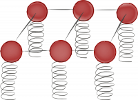
The formalism of quantum field theory is quite similar to how we treat the harmonic oscillator in quantum mechanics. The picture below nicely summarizes the analogies.

Abstract

In the quantum case, axiomatic formulations of field theory assert that fields $\varphi$ are operator-valued distributions [8]. Distributions are continuous linear functionals which map a space of test functions $\mathcal{T}$ onto the complex numbers: $\varphi: \mathcal{T} \rightarrow \mathbb{C}$. In quantum field theory (QFT), $\mathcal{T}$ is chosen to be some set of space-time functions; usually either the space of continuous functions with compact support $\mathcal{D}(\mathbb{R}^{1,3})$, or the space of Schwartz functions $\mathcal{S}(\mathbb{R}^{1,3})$. (The distributions with which these test functions are smeared are called tempered distributions.) In either of these cases one can represent the image of the map $\varphi$ on a space-time function $f$ as: \begin{align} \varphi(f) = (\varphi,f) : = \int d^{4}x \ \varphi(x)f(x) \label{int_rep} \end{align} which gives meaning to the $x$-dependent field expression $\varphi(x)$. Since $\varphi$ is an operator-valued distribution in QFT, only the smeared expression $\varphi(f)$ is guaranteed to correspond to a well-defined operator. The derivative of a distribution $\varphi'$ is defined by: \begin{align} (\varphi',f) := -(\varphi,f') \end{align} and is itself also a distribution [8]. By applying the integral representation in equation~\ref{int_rep}, one can interpret this definition as an integration by parts where the boundary terms have been `dropped': \begin{align} \int d^{4}x \ \varphi'(x)f(x) = -\int d^{4}x \ \varphi(x)f'(x) \end{align} Although this shorthand notation is useful, and will be used for the calculations in this paper, it can also be slightly misleading. Sometimes it is incorrectly stated that integration by parts of quantum fields can be performed, and the boundary terms neglected. However, distributions are generally not point-wise defined, so boundary expressions like: $\int_{\partial \mathbb{R}^{3} } \varphi(x)f(x)$ are often ill-defined. Therefore, when manipulations like this are performed one is really just applying the definition of the derivative of a distribution, there are no boundary contributions. This makes the question of whether spatial boundary term operators vanish a more subtle issue in QFT than in the classical case.

The physical rationale behind using operator-valued distributions as opposed to operator-valued functions in QFT is because operators inherently imply a measurement, and this is not well-defined at a single (space-time) point since this would require an infinite amount of energy [9]. Instead, one can perform a measurement over a space-time region $\mathcal{U}$, and model the corresponding operator $\mathcal{A}(f)$ as a distribution $\mathcal{A}$ smeared with some test function $f$ which has support in $\mathcal{U}$. If one were to smear $\mathcal{A}$ with another test function $g$, which has different support to $f$, then in general the operators $\mathcal{A}(f)$ and $\mathcal{A}(g)$ would be different. But the interpretation is that these operators measure the same quantity, just within the different space-time regions: $\text{supp}(f)$ and $\text{supp}(g)$.

As well as differentiation it is also possible to extend the notion of multiplication by a function to distributions. Given a distribution $\varphi$, a test function $f$, and some function $g$, this is defined as: \begin{align} (g\varphi,f) := (\varphi,gf) \label{dist_prop} \end{align} In order that $g\varphi$ defines a distribution in the case where $f\in \mathcal{D}$, it suffices that $g$ be an infinitely differentiable function. For tempered distributions, in which $f\in \mathcal{S}$, it is also necessary that $g$ and all of its derivatives are bounded by polynomials [8].

Besides the assumption that fields are operator-valued distributions, axiomatic approaches to QFT usually postulate several additional conditions that the theory must satisfy. Although different axiomatic schemes have been proposed, these schemes generally contain a common core set of axioms\footnote{See[8] ,[9] and [10] for a more in-depth discussion of these axioms and their physical motivation.}. For the purpose of the calculations in this paper, the core axioms which play a direct role are: ….

Generally the product of distributions is not well-defined, and so one must first introduce a regularisation procedure in order to make sense of such products [9].

[…]

a property which is well-established in Quantum Electrodynamics (QED) [14], as well as other gauge theories [15] – charged states are non-local. This means that it is not possible to create a charged state by applying a local operator to the vacuum. However, by virtue of the Reeh–Schlieder Theorem, a charged state can always be approximated by local states as closely as one likes in the sense of convergence in some allowed topology on H. Often this topology is chosen to be the weak topology and so convergence means weak convergence.

Boundary terms in quantum field theory and the spin structure of QCD by Peter Lowdon

The comment regarding the impossibility to create a charged state using local operators is true because gauge interactions have infinite reach. E.g. the photon is massless and thus an electrically charged particle, like an electron, is always surrounded by a cloud of photons, even infinitely far away. In this context a charged particle is called an infraparticle.

see the discusssion about "Quantum Field Theory from a mathematical point of view" at StackExchange

Useful Introductions:

For a nice overview, see "What is Quantum Field Theory", by Yuji Tachikawa
and in particular How I Learned to Stop Worrying and Love QFT by Mario Flory
and An introduction to rigorous formulations of quantum field theory by Ranard

Why is it interesting?

Quantum field theory is the best theory of fundamental interactions that we have. It allows us to compute the probability that certain new particles are created if we smash two particles, for example electrons, together

Most importantly, it allows us to understand how particles can be described in a field theory.

Everything in nature is some field configuration.Urs Schreiber

"There are no particles, there are only fields" https://arxiv.org/abs/1204.4616

In its mature form, the idea of quantum field theory is that quantum fields are the basic ingredients of the universe, and particles are just bundles of energy and momentum of the fields. In a relativistic theory the wave function is a functional of these fields, not a function of particle coordinates. Quantum field theory hence led to a more unified view of nature than the old dualistic interpretation in terms of both fields and particles. What is Quantum Field Theory, and What Did We Think It Is? by S. Weinberg

We have no better way of describing elementary particles than quantum field theory. A quantum field in general is an assembly of an infinite number of interacting harmonic oscillators. Excitations of such oscillators are associated with particles. The special importance of the harmonic oscillator follows from the fact that its excitation spectrum is additive, i.e. if $E_1$ and $E_2$ are energy levels above the ground state then $E_1 + E_2$ will be an energy level as well. It is precisely this property that we expect to be true for a system of elementary particles. A. M. Polyakov, “Gauge Fields and Strings”, 1987

Undoubtedly the single most profound fact about Nature that quantum field theory uniquely explains is the existence of different, yet indistinguishable, copies of elementary particles. Two electrons anywhere in the Universe, whatever their origin or history, are observed to have exactly the same properties. We understand this as a consequence of the fact that both are excitations of the same underlying ur-stuff, the electron field. Quantum Field Theory by Frank Wilczek

For further motivation for quantum field theory, see also https://arxiv.org/abs/hep-th/9803075
and for an especially nice discussion of the question "Why Quantum Field Theory?" see page 5ff in http://www.damtp.cam.ac.uk/user/tong/qft/qft.pdf

FAQ

For many more questions and answers see: http://www.mat.univie.ac.at/~neum/physfaq/physics-faq.html

In what sense is a quantum field an infinite set of harmonic oscillators?: see also https://physics.stackexchange.com/questions/127141/in-what-sense-is-a-quantum-field-an-infinite-set-of-harmonic-oscillators

What does QFT “get right” that QM “gets wrong”?: See https://physics.stackexchange.com/questions/31635/what-does-qft-get-right-that-qm-gets-wrong/31648#31648

What kind of infinites arise in QFT?: See https://physics.stackexchange.com/questions/70411/the-divergence-in-qcd-series-how-many-are-they-and-what-do-they-mean/70420#70420

Why are fields in QFT operator valued DISTRIBUTIONS and not operator valued FUNCTIONS?: The physical rationale behind using operator-valued distributions as opposed to operator valued functions in QFT is because operators inherently imply a measurement, and this is not well-defined at a single (space–time) point since this would require an infinite amount of energy [9]. Instead, one can perform a measurement over a space–time region U, and model the corresponding operator A(f) as a distribution A smeared with some test function f which has support in U. If one were to smear A with another test function g, which has different support to f , then in general the operators A(f ) and A(g) would be different. But the interpretation is that these operators measure the same quantity, just within the different space–time regions: supp(f ) and supp(g).

Boundary terms in quantum field theory and the spin structure of QCD by Peter Lowdon

In what sense has a quantum field infinitely many degrees of freedom?: Speaking colloquially, we have a harmonic oscillator at each spacetime point. With the standard assumption of a continuous spacetime time, we can therefore conclude that we have infinitely many harmonic oscillators in any finite spacetime-volume. These correspond to the infinitely many degrees of freedom.

Is Quantum Field Theory mathematically consistent?

Strictly speaking, quantum field theory (at least in most of the fully relevant non-trivial instances of this theory that we know is mathematically inconsistent, and various 'tricks' are needed to provide meaningful calculational operations. It is a very delicate matter to know whether these tricks are merely stop-gap procedures that enable us to edge forward with an mathematical framework that may perhaps be fundamentally flawed at a deep level, or whether these tricks reflect profound truth that actually have a genuine significance to Nature herself. Most of the recent attempts to move forward in fundamental physics indeed take many of these 'tricks' to be fundamental.

page 610 in Road to Reality by R. Penrose

Common signs of mathematical problems in QFT are that the perturbation series does not converge and that we need renormalization procedures to get rid of infinites. However, these problems are actually not as severe as they may seem.

The non-convergence of the perturbation series can be traced back to the fact that the perturbation theory does not include contributions from non-perturbative effects, like instantons.

The appearance of infrared divergences can be traced back to our simplified assumption that spacetime is infinite.

Lastly and most importantly, one can show that the appearance of ultraviolet divergences has its origin in the fact that we physicists handle Distributions improperly.

For more on this, have a look at: How I Learned to Stop Worrying and Love QFT by Robert C. Helling.

What is the connection to statistical Mechanics?: https://mcgreevy.physics.ucsd.edu/s14/239a-lectures.pdf

What is the Cluster Decomposition Principle?

This principle says that distant processes do not affect each other. In this sense it is the weakest form of locality and it necessary if we want to talk about well-separated particles.

This property of QFTs is emphasized by Weinberg in his QFT books.

Weinberg's view of QFT is nicely summarized in chapter 2 of http://sites.krieger.jhu.edu/jared-kaplan/files/2016/05/QFTNotes.pdf

Can every QFT be described by a Lagrangian?

No!

Basically, all the textbooks on quantum field theories out there use an old framework that is simply too narrow, in that it assumes the existence of a Lagrangian.

This is a serious issue, because when you try to come up e.g. with a theory beyond the Standard Model, people habitually start by writing a Lagrangian … but that might be putting too strong an assumption.

We need to do somethingWhat is Quantum Field Theory by Yuji Tachikawa

See also https://youtu.be/XM4rsPnlZyg?t=9m32s around 9:30

It is good to keep in mind, as much as physicists love Lagrangians, there are many many very interesting theories that you can almost prove that there is no Lagrangian description for them. That's kind of a warning sign that if you really want to understand quantum field theory, a Lagrangian cannot be the starting point. Duality and emergent gauge symmetry - Nathan Seiberg

The Lagrangian approach is good for approximations and to get a geometric point of view. Whereas a description without a Lagrangian, i.e. in terms of operators and correlation functions is useful for exact solutions and yields an algebraic point of view.

There is a lot of evidence that probably neither of them will end up to be the fundamental one. Duality and emergent gauge symmetry - Nathan Seiberg

Is there a unique Lagrangian for each Quantum Field Theory?: No! See https://youtu.be/XM4rsPnlZyg?t=10m44s around 10:44

There are many theories, which have more than one Lagrangian. So that's the opposite. Either we have no Lagrangian at all or we have more than one Lagrangian.

Duality and emergent gauge symmetry - Nathan Seiberg