Spin Models

Prerequisites: Statistical Mechanics, Spin. Full path (22 pages)

Intuitive
Concrete
Abstract
Overview
Why is interesting?

Intuitive

A bar magnet is made of a huge number of atoms, and each atom behaves like a tiny compass needle, a spin. Neighbouring spins in a ferromagnet prefer to point in the same direction. Heat works against this: thermal motion flips the spins at random. At low temperature the alignment wins, most spins point the same way and the material is magnetised. Above a critical temperature the random flipping wins and the magnetisation disappears. Between the two there is a phase transition.

A spin model throws away almost everything about the real material and keeps only this competition. We put an arrow on every site of a regular grid, give the system lower energy when neighbouring arrows agree, and ask what the arrows do at a given temperature. Models differ in what an arrow is allowed to do: point only up or down, point in one of a few fixed directions, or point in any direction in a plane or in space.

The surprise is how much these crude models get right. Close to a phase transition the behaviour of very different systems, a uniaxial magnet, a liquid near its critical point, a mixture of two metals, is described by the same numbers (critical exponents). These numbers depend only on the dimension of space and on the symmetry of the arrows, not on the microscopic details. So a simple spin model on a grid can describe a real system quantitatively near its critical point. Spin models are also the standard test case for methods of statistical mechanics, from exact solutions to computer simulations and the renormalization group.

Concrete

A spin model is defined by a lattice (for example $\mathbb{Z}^d$ ), a set of allowed values for the spin at each site, and an energy function $\mathcal{H}$ . All thermal properties follow from the partition function

$Z = \sum_{\{\text{configurations}\}} e^{-\beta \mathcal{H}}, \qquad \beta = \frac{1}{k_B T},$

and the free energy $F = -k_B T \ln Z$ .

Ising model. Each site carries $s_i \in \{+1,-1\}$ and

$\mathcal{H} = -J \sum_{\langle ij\rangle} s_i s_j - h\sum_i s_i ,$

where $\langle ij \rangle$ runs over nearest-neighbour pairs, $J > 0$ favours alignment and $h$ is an external magnetic field. The order parameter is the magnetisation per site $m = \langle s_i \rangle$ .

Example: the one-dimensional chain. For a ring of $N$ sites, write $e^{-\beta\mathcal H}$ as a product of factors that each involve two neighbouring spins. Then $Z = \text{Tr}\, \mathsf{T}^N$ with the transfer matrix

$\mathsf{T} = \begin{pmatrix} e^{\beta(J+h)} & e^{-\beta J} \\ e^{-\beta J} & e^{\beta(J-h)} \end{pmatrix}.$

At $h = 0$ its eigenvalues are $\lambda_+ = 2\cosh\beta J$ and $\lambda_- = 2\sinh \beta J$ , so $Z = \lambda_+^N + \lambda_-^N$ and for large $N$ the free energy per site is $f = -k_B T \ln(2\cosh\beta J)$ . This is analytic for all $T > 0$ : the one-dimensional Ising model has no phase transition. The correlation length $\xi = 1/\ln(\lambda_+/\lambda_-)$ in units of the lattice spacing is finite at every $T>0$ and diverges only as $T \to 0$ .

In two dimensions the model does order. Onsager's exact solution on the square lattice gives the critical temperature from $\sinh(2J/k_B T_c) = 1$ , that is $k_B T_c = 2J/\ln(1+\sqrt{2}) \approx 2.269\, J$ .

Mean field approximation. Replace the neighbours of a spin by their average $m$ . A spin then sees an effective field $zJm + h$ , where $z$ is the number of nearest neighbours, and self-consistency requires $m = \tanh\big(\beta(zJm + h)\big)$ . At $h=0$ a non-zero solution exists for $k_B T < zJ$ . Mean field theory predicts a transition in every dimension, which is wrong for $d=1$ , and its critical exponents are correct only for $d \geq 4$ (with logarithmic corrections at $d = 4$ ).

Potts and n-vector models. In the $Q$ -state Potts model $\chi_i \in \{1,\dots,Q\}$ and $\mathcal{H} = -J\sum_{\langle ij\rangle} \delta(\chi_i,\chi_j)$ . For $Q = 2$ , writing $\delta(\chi_i,\chi_j) = \frac{1}{2}(1 + s_i s_j)$ shows that it is the Ising model with coupling $J/2$ . In the n-vector model $\vec S_i$ is a unit vector in $\mathbb{R}^n$ and $\mathcal{H} = -J\sum_{\langle ij \rangle}\vec S_i\cdot\vec S_j$ . The cases $n = 1, 2, 3$ are the Ising, XY and classical Heisenberg models. For $n \geq 2$ the symmetry is continuous, and the Mermin-Wagner theorem rules out spontaneous magnetisation at $T > 0$ in $d \le 2$ for short-range interactions. The two-dimensional XY model still has a transition of a different kind, the Berezinskii-Kosterlitz-Thouless transition, driven by the unbinding of vortices.

Abstract

A classical spin model consists of a countable graph $\Lambda$ (typically $\mathbb{Z}^d$ with nearest-neighbour edges), a single-spin space $S$ with an a priori probability measure $\mu_0$ (a finite set with counting measure for Potts models, the sphere $S^{n-1}$ with its round measure for n-vector models), and an interaction, a family of functions $\Phi_A$ on $S^A$ for finite $A \subset \Lambda$ . A symmetry group $G$ acts on $S$ preserving $\mu_0$ and $\Phi$ : $S_Q$ for the Potts model and $O(n)$ for the n-vector model.

Gibbs measures and phase transitions. In finite volume the Gibbs measure is $\mu(d\sigma) \propto e^{-\beta \mathcal{H}(\sigma)} \prod_i \mu_0(d\sigma_i)$ . In infinite volume one defines Gibbs measures on $S^\Lambda$ by the Dobrushin-Lanford-Ruelle condition: the conditional distribution in every finite region, given the configuration outside, is the finite-volume Gibbs measure with those boundary conditions. The set of Gibbs measures at given $\beta$ is a convex set (a simplex), and its extremal points are the pure phases. Phase coexistence, the sense of phase transition used in this setting, is the existence of more than one Gibbs measure. Spontaneous symmetry breaking means that the extremal Gibbs measures are not $G$ -invariant, even though the set of them is. For the Ising model in $d \ge 2$ the Peierls contour argument proves non-uniqueness at low temperature, with the $+$ and $-$ phases selected by boundary conditions.

Random cluster representation. Writing $e^{\beta J\delta(\chi_i,\chi_j)} = e^{\beta J}\left[(1-p) + p\,\delta(\chi_i,\chi_j)\right]$ with $p = 1 - e^{-\beta J}$ and expanding the product over the edge set $E$ of a finite graph gives the Fortuin-Kasteleyn representation

$Z_{\text{Potts}} = e^{\beta J |E|}\sum_{A\subseteq E} p^{|A|}(1-p)^{|E|-|A|}\, Q^{k(A)},$

where $k(A)$ is the number of connected components of the graph $(\Lambda, A)$ , isolated vertices included. The right hand side makes sense for any real $Q > 0$ , and $Q \to 1$ gives bond percolation. Spontaneous magnetisation of the Potts model corresponds to percolation of the random clusters.

Dualities, transfer matrices and continuum limits. The transfer matrix maps a classical model in $d$ dimensions to a quantum spin chain or lattice in $d-1$ dimensions; the two-dimensional Ising model corresponds to the one-dimensional transverse-field Ising chain. On the square lattice, Kramers-Wannier duality relates the Ising model at couplings $K = \beta J$ and $K^*$ with $\sinh 2K \sinh 2K^* = 1$ , and the self-dual point is the critical point found by Onsager. Near a continuous transition the long-distance behaviour is governed by a fixed point of the renormalization group. For the n-vector model this is the $O(n)$ -symmetric $\phi^4$ field theory, with the Gaussian fixed point above the upper critical dimension $d = 4$ and the Wilson-Fisher fixed point below it. In $d = 2$ the critical points are described by conformal field theories; the critical Ising model is the minimal model with central charge $c = \frac{1}{2}$ .

Overview

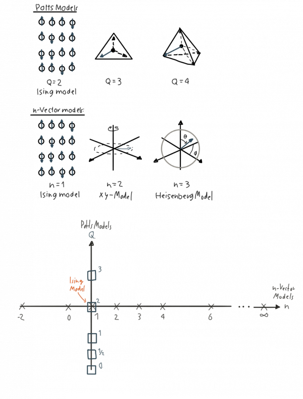
Spin models can be classified depending on how many different states are possible at each lattice site and if the set of possible states is continuous or discrete.

Models with a discrete set of states are called Potts models.
Models with a continuous set of states are called n-Vector models.

Within these subcategories we have different models depending on how many states there are in total. For Potts models, the number of orientations that are possible is denoted by $Q$ . For n-vector models, the dimension in which the continuous set of states live at each node is denoted by an $n$ .

For $n=1$ and $Q=2$ the two types of models overlap and this special model is known as the Ising model.

The first of these is the Q-state Potts model (Potts, 1952; Wu, 1982). One assumes that each spin i can be in one of Q possible discrete orientations $\chi_i$ $(\chi_i =1,2,\ldots,Q)$ . If two neighboring spins i and j are in the same orientation, then they contribute an amount $-J$ to the total energy of a configuration. If i and j are in different orientations, they contribute nothing. Thus the interaction Hamiltonian is

$\mathcal H(d,s)=-J\sum_{\langle ij\rangle} \delta(\chi_i, \chi_j)$

where $\delta(\chi_i ,\chi_j)=1$ if $\chi_i=\chi_j$ , and is zero otherwise. The angular brackets in Eq. (12a) indicate that the summation is over all pairs of nearest-neighbor sites $\langle ij\rangle$ . The interaction energy of a pair of neighboring parallel spins is $-J$ , so that if $J>0$ , the system should order ferromagnetically at $T=0$ .

The second such model is the n-vector model (Stanley, 1968), characterized by spins capable of taking on a continuum of states. The Hamiltonian for the n-vector model is

$\mathcal H(d,n)=-J\sum_{\langle ij\rangle} \vec S_i \cdot \vec S_j$ Here, the spin $\vec S_i=(S_{i1} ,S_{i2} ,\ldots,S_{in})$ is an n-dimensional unit vector with ( $\sum_{\alpha=1}^n S_{i\alpha}^2=1$ , and $\vec S_i$ interacts isotropically with spin $\vec S_j$ localized on site j. Two parameters in the n-vector model are the system dimensionality d and the spin dimensionality n. The parameter n is sometimes called the order-parameter symmetry number; both d and n determine the universality class of a system for static exponents. Both the Potts and n-vector hierarchies are generalization of the simple Ising model of a uniaxial ferromagnet. Scaling, universality, and renormalization: Three pillars of modern critical phenomena by H.Eugene Stanley

Why is interesting?

"Empirically, one finds that all systems in nature belong to one of a comparatively small number of such universality classes. Two specific microscopic interaction Hamiltonians appear almost sufficient to encompass the universality classes necessary for static critical phenomena.

[…] [T]he Q-state Potts model (Potts, 1952; Wu, 1982) [and] the n-vector model (Stanley, 1968).

Scaling, universality, and renormalization: Three pillars of modern critical phenomena by H.Eugene Stanley

Phase transitions are a central theme of statistical mechanics, and of probability more generally. Lattice spin models represent a general paradigm for phase transitions in finite dimensions, describing ferromagnets and even some fluids (lattice gases).Lectures on the Ising and Potts models on the hypercubic lattice by Hugo Duminil-Copin

Contributing authors:

Path to this page

Authors: Jakob Schwichtenberg