Schrödinger Equation

Prerequisites: Hamiltonian Formalism, Imaginary Numbers. Full path (14 pages)

Best explanations

Concrete Feynman's derivation of the Schrödinger equation

Intuitive
Concrete
Abstract
Why is it interesting?
Research
Definitions
FAQ
History

$\color{royalblue}{i} \color{olive}{\hbar} \color{darkturquoise}{\partial_t} \color{firebrick}{\Psi(\vec{x},t)} = \color{darksalmon}{\hat H} \color{firebrick}{\Psi(\vec{x},t)}$

see also Quantum Mechanics

Intuitive

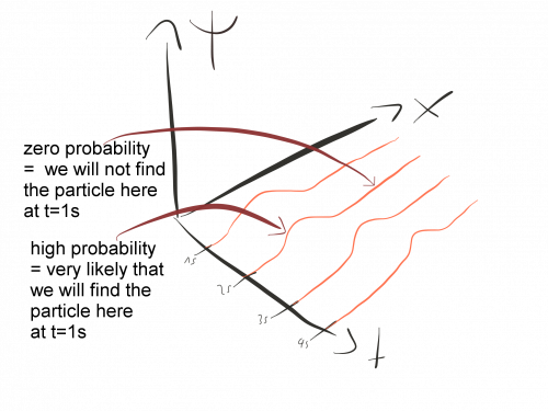
The Schrödinger equation describes how the state of a quantum system changes in time. It is as central to quantum mechanics as Newton’s laws are to classical mechanics

In quantum mechanics, we describe particles using waves. However, these waves are not waves in the same sense as sound waves or ocean waves. Rather, they are probability waves that tell us where it is likely to find a given particle.

Every time in physics we describe something in terms of waves, we need a wave equation that tells us how the waves behave in different situations. The Schrödinger equation is the correct equation to describe the probability waves of quantum mechanics.

The Schrödinger equation tells us that rate of change of the wave-function is completely determined by the total energy of the system.

In addition, it tells us that the wave-function is a complex function. Therefore, it cannot represent anything in our real world like, for example, a spatial displacement. Instead, to get something that gets actually measured in experiments, we must consider the absolute value of the wave function, which then represents the probability that something happens.

It also tells us that the actual size of quantum effects is tiny.

While in principle, Schrödinger's equation enables us to describe any kind of quantum system this is in practice quite hard. We can solve the Schrödinger equation only for very special simplified systems. For all other systems, approximation methods must be used.

Concrete

In the Schrödinger equation, the wave-function $\color{firebrick}{\Psi(\vec{x},t)}$ describes the state of the system. This means concretely that ${ \Psi(\vec{x},t)}$ encodes, for example, if a given system is excited or in its rest state. The wave-function is a complex function, which means that at a given point in space, say $\vec{x}= (1,4,7)$ , and time, say $t=9s$ , the wave function is a complex number: ${\Psi(1,4,7,9)}= 5 + 3 i$ . The wave-function at a given point in space and time yields a probability amplitude. By taking the absolute square of an probability amplitude we get the probability density and by integrating over some spatial volume we get the probability of the particle being within this volume.

The left-hand side of the Schrödinger equation denotes the of the wave function. We act with the partial derivative $\color{darkturquoise}{\partial_t}$ on our wave-function and the result: ${\partial_t}{ \Psi(\vec{x},t)}$ denotes how the wave function changes as time passes on.

The Hamiltonian operator $\color{darksalmon}{\hat H}$ represents the total energy of the system. We can get the Hamiltonian operator from the classical energy $E= T +V$ , where $T$ is the kinetic energy and $V$ the potential energy by replacing

$\begin{align} \text{ the classical momentum } p_i \ &\rightarrow \ {-i} \hbar \partial_{x_i} \, . \end{align}$

Formulated differently, the Hamiltonian operator is calculated from the classical energy $E= T +V$ by replacing the classical momentum $p_i$ with the momentum operator $\hat{p}_i \equiv {-i} \hbar \partial_{x_i}$ :

$\begin{equation} \hat H \equiv - \frac{\hbar^2}{2m} \nabla^2 + \hat V \hat{=} \frac{\hat{p}^2}{2m} + \hat V. \end{equation}$

It is conventional to denote operators by an additional hat above the classical symbol.

The Hamiltonian is what is different for different systems. Formulated differently, the Hamiltonian characterizes the system in question. The rest of the Schrödinger equation stays the same for all systems. For example, the Hamiltonian for a harmonic oscillator reads

$\begin{equation} \hat H \equiv \frac{\hat{p}^2}{2m} + \frac{1}{2}k \hat{x}^2 . \end{equation}$

Stationary Schrödinger equation

For systems with a time-independent Hamiltonian $\partial_t H =0$ , it is helpful to split the wave function into two parts $\Psi(x,t) = \phi(t) \psi(x)$ . We can see why this is useful by putting this ansatz into the Schrödinger equation

$\begin{align} i \hbar \partial_t \Psi(x,t) &= H \Psi (x,t) \\ i \hbar \partial_t\phi(t) \psi(x) &= H \phi(t) \psi(x) \\ i \hbar \frac{\partial_t \phi(t)}{\phi(t)} &= \frac{H \psi(x)}{\psi(x)} . \end{align}$ Take note that Hamiltonian $H$ on the right-hand side contains the momentum operator $i \partial_{x}$ and thus $\psi(x)$ does not cancel here. The left-hand side now only depends on $t$ while the right-hand side only depends on $x$ . This equation can only be correct for arbitrary values for $x$ and arbitrary values for $t$ when both sides independently yield some constant that we call $E$ : $\begin{align} \Rightarrow \quad i \hbar \frac{\partial_t \phi(t)}{\phi(t)} &= E , \Rightarrow\frac{H \psi(x)}{\psi(x)} &= E. \end{align}$

The solution of the first equation is

$\phi(t) = A e^{-Et/\hbar}$ and the second equation is known as the stationary Schrödnger equation. This means that for all systems where the Hamiltonian does not explicitly depend on the time, we know immediately what the time-dependence of the total wave function $\Psi(x,t)$ looks like, namely: $\Psi(x,t) = \phi(t) \psi(x) = A e^{-Et/\hbar} \psi(x)$ . The only thing we then have to do is to solve the stationary Schrödinger equation

$\begin{equation} \colorbox{lightpink}{$H \psi(x)= E\psi(x)$} \end{equation}$ for the Hamiltonian $H$ that describes the system in question.

The complete wave function then reads

$\colorbox{lightpink}{${\Psi(x,t) = \phi(t) \psi(x) = A e^{-Et/\hbar} \psi(x)}$}$

Example: Free Particle

The Hamiltonian for a free particle is $H= \frac{-\hbar \partial_x^2}{2m}$ . The stationary Schrödinger equation therefore reads

$\begin{align} H \psi(x)&= E\psi(x) \\ \frac{-\hbar \partial_x^2}{2m} \psi(x) &=E\psi(x) \end{align}$ This equation is solved for $E>0$ by

$\Psi(x) =A e^{i\sqrt{2mE/\hbar}x} + B e^{-i\sqrt{2mE/\hbar}x}.$

Such a solution describes a plane wave. However, since such a plane wave solution cannot be normalized (which we need since the total probability has to be 100\%), it is not a physical solution. Instead, to describe a real free particle we need to use a normalizable superposition of such plane wave solutions that we call wave packets.

Wave Packets

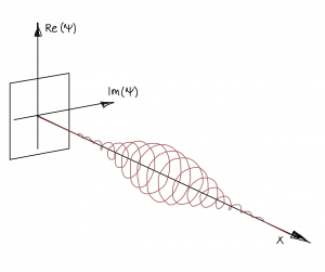
A generic solution of the stationary Schrödinger equation

$\Psi(x) =A e^{i\sqrt{2mE/\hbar}x} + B e^{-i\sqrt{2mE/\hbar}x}$

is non-physical, since it describes a plane wave that oscillates till infinity and therefore can't be normalized.

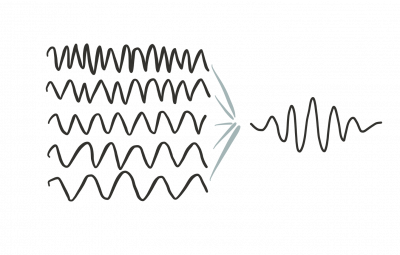
To get something that we can normalize we must use a superposition of such generic solutions. By adding plane waves with different oscillation frequencies we can build a wave packet that is localized in space and therefore can be normalized.

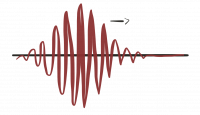
One possibility is a Gaussian wave-packet, where $A(\vec p)$ is a Gauss distribution. $\Psi_{GWP}( \vec x,t) = \int d p^3 A(\vec p) e^{i( \vec p \vec x-Et)} = \int d p^3 \psi_0 e^{i(\vec p-\vec{ \tilde p})^2/4\sigma^2} {\mathrm{e }}^{i( \vec p \vec x-Et)} \, .$

Take note that using a Fourier transform a wave packet can be tought of as being built of plane waves:

Examples

One of the most important examples is the particle in a box, since it demonstrates nicely how the quantization of energy levels happens in quantum mechanics.

Particle in a box

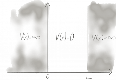
A particle confined in a box, here 1-dimensional, with infinitely high potential walls is one of the standard examples of quantum mechanics. Inside the box the potential is zero, outside it's infinite.

The potential is defined piece-wise

$\begin{equation} V = \left\{ \begin{array}{ll} 0, & 0< x <L \\ \infty, & {\mathrm{\ otherwise }} \end{array} \right. \end{equation}$ and therefore, we have to solve the one-dimensional Schrödinger equation piece-wise. $i \partial_t \Psi(\vec{x},t) = -\frac{\partial_x^2}{2m} \Psi(x,t) + V(x) \Psi(x,t)$

Inside the box, the solution is equal to the free particle solution, because $V=0$ for $0< x <L$
Outside, because $V=\infty$ , the only possible, physical solution is $\Psi(x,t)=0$ .

We can rewrite the general free particle solution $\Psi(x,t) = A {\mathrm{e }}^{-i ( E t - \vec p \cdot \vec x) } + B {\mathrm{e }}^{-i ( E t + \vec p \cdot \vec x) }$ $= \big( C \sin(\vec p \cdot \vec x) + D \cos(\vec p \cdot \vec x) \big){\mathrm{e }}^{-i E t},$ which we can rewrite again using the non-relativistic energy-momentum relation $E = \frac{\vec{p}^2}{2m} \qquad \rightarrow \qquad \vec p = \sqrt{2mE}$ $\begin{equation} \Psi(x,t) = \big( C \sin(\sqrt{2mE}x) + D \cos(\sqrt{2mE}x) \big){\mathrm{e }}^{-i E t} \end{equation}$

Next, we use that the wave-function must be a continuous function¹. Therefore, we have the boundary conditions $\Psi(0)=\Psi(L) \stackrel{!}{=} 0$ . We see that, because $\cos(0)=1$ we have $D\stackrel{!}{=}0$ . Furthermore, we see that these conditions impose $\begin{equation} \sqrt{2mE}\stackrel{!}{=} \frac{n \pi}{L}, \end{equation}$ with arbitrary integer $n$ , because for ²

$\begin{equation} \Phi_n(x,t)=C\sin(\frac{n \pi}{L} x){\mathrm{e }}^{-i E_n t} \end{equation}$ both boundary conditions are satisfied $\rightarrow \Phi_n(L,t)=C\sin(\frac{n \pi}{L} L){\mathrm{e }}^{-i E t} = C\sin(n \pi){\mathrm{e }}^{-i E t} =0 \qquad \checkmark$ $\rightarrow \Phi_n(0,t)= C \sin(\frac{n \pi}{L} 0){\mathrm{e }}^{-i E t} = C\sin(0){\mathrm{e }}^{-i E t} =0 \qquad \checkmark$ The normalization constant $C$ , can be found to be $C=\sqrt{\frac{2}{L}}$ , because the probability for finding the particle anywhere inside the box must be $100\%=1$ and the probability outside is zero, because there we have $\Psi=0$ . Therefore $P= \int_0^L dx \Phi_n^\star(x,t) \Phi_n(x,t) \stackrel{!}{=} 1$ $P = \int_0^L dx C^2 \sin(\frac{n \pi}{L} x){\mathrm{e }}^{+i E t} \sin(\frac{n \pi}{L} x){\mathrm{e }}^{-i E t}$ $= C^2 \int_0^L dx \sin^2(\frac{n \pi}{L} x) = C^2 \left[\frac{x}{2} -\frac{\sin (\frac{2n \pi}{L} x)}{4 \frac{n \pi}{L}} \right]_0^L$ $= C^2 \left( \frac{L}{2} - \frac{\sin (\frac{2n \pi}{L} L)}{4 \frac{n \pi}{L}} \right) = C^2 \frac{L}{2} \stackrel{!}{=} 1$ $\rightarrow C^2 \stackrel{!}{=} \frac{2}{L} \qquad \checkmark$ We can now solve Eq.~\ref{box:quantbed} for the energy $E$

$\begin{equation} E_n \stackrel{!}{=} \frac{n^2 \pi^2}{L^2 2m}. \end{equation}$ The possible energies are quantized, which means that the corresponding quantity can only be integer multiplies of some constant, here $\frac{ \pi^2}{L^2 2m}$ . Hence the name quantum mechanics.

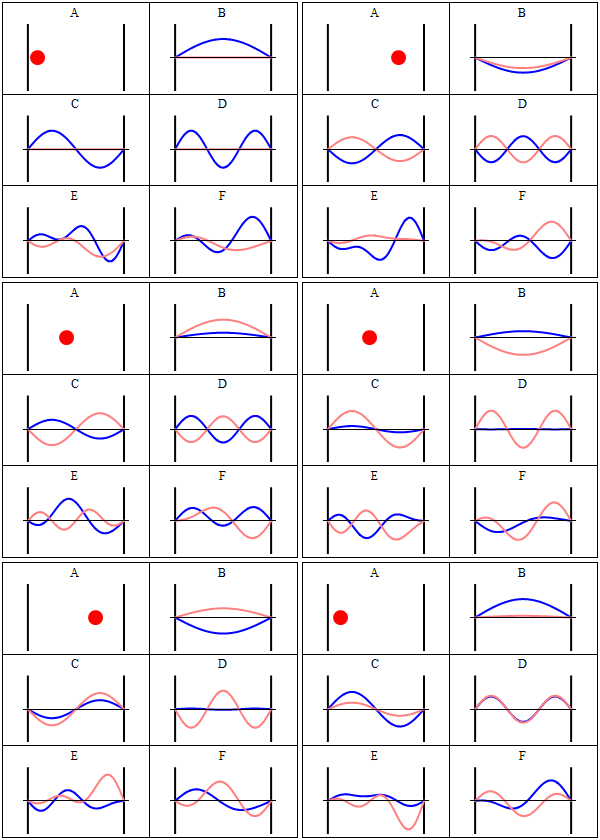
$A$ shows a solution of the particle in a box system in classical mechanics. $B-F$ show quantum mechanical solutions.

Take note that we have a solution for each $n$ and linear combinations of the form $\Phi(x,t) = A \Phi_1(x,t) + B \Phi_2(x,t) + \ldots$ are solutions, too. These solutions have to be normalised again because of the probabilistic interpretation³.

See also Feynman's derivation of the Schrödinger equation.
Moreover it can be derived by using the symmetry group of non-relativistic physics, i.e. the Galilei group. This is shown at page 209 in Josef M. Jauch: "Foundations of Quantum Mechanics".
The Schrödinger equation is the non-relativistic limit of the Klein-Gordon equation. (This is shown, for example, in Physics from Symmetry by Schwichtenberg)
No-Nonsense Quantum Mechanics by Jakob Schwichtenberg, section "How Quantum Systems Change"

Abstract

The state of a quantum system is a unit vector $\Psi$ in a complex separable Hilbert space $\mathcal H$ , defined up to a phase, and the Hamiltonian $\hat H$ is a self-adjoint operator on a dense domain $D(\hat H)\subset\mathcal H$ . For a time-independent $\hat H$ , Stone's theorem gives a one-to-one correspondence between self-adjoint operators and strongly continuous one-parameter groups of unitary operators,

$\hat U(t) = e^{-i\hat H t/\hbar} ,$

defined through the spectral theorem. The solution of the Schrödinger equation with initial state $\Psi_0$ is $\Psi(t) = \hat U(t)\Psi_0$ . If $\Psi_0 \in D(\hat H)$ , then $\Psi(t)\in D(\hat H)$ for all $t$ and $\Psi(t)$ is differentiable in the norm of $\mathcal H$ , with $i\hbar\,\frac{d}{dt}\Psi(t) = \hat H\Psi(t)$ . For other $\Psi_0$ the unitary evolution is still defined, and the equation holds in a weak sense. Conversely, if the dynamics is a continuous unitary group, the generator is self-adjoint, so the Schrödinger equation is the infinitesimal form of a continuous unitary representation of the group of time translations $(\mathbb R,+)$ .

This is why self-adjointness, and not only symmetry ( $\langle\phi,\hat H\psi\rangle = \langle\hat H\phi,\psi\rangle$ on the domain), is the condition that matters. A symmetric operator can have several self-adjoint extensions, which give different dynamics and correspond physically to different boundary conditions. For $\hat H = -\frac{\hbar^2}{2m}\Delta + V$ on $L^2(\mathbb R^3)$ , the Kato-Rellich theorem shows that $\hat H$ is self-adjoint on the domain of the Laplacian whenever $V$ is relatively bounded with respect to $\Delta$ with relative bound less than one. This covers the Coulomb potential and hence the hydrogen atom.

Since states are rays, what is fixed by symmetry is only a projective representation. For the Galilei group, the unitary representations needed are those of a central extension in which the mass is the central charge (Bargmann), and the free Schrödinger equation is the equation of motion of these representations.

The equation also has a Hamiltonian form. Viewed as a real vector space, $\mathcal H$ is symplectic with symplectic form proportional to $\mathrm{Im}\langle\cdot,\cdot\rangle$ , and the Schrödinger equation is the flow of the Hamiltonian function $\Psi\mapsto\langle\Psi,\hat H\Psi\rangle$ . The flow descends to the projective Hilbert space, a Kähler manifold with the Fubini-Study metric. In this form the linear Schrödinger equation is a special case of a symplectic Hamiltonian system whose Hamiltonian is quadratic.

One way to state the Schrödinger equation is that: "Energy is the operator that infinitesimally generates time translations". (Source)

Why is it interesting?

The Schrödinger equation is the basic equation of motion in quantum mechanics and also describes the time evolution of states in quantum field theory.

In quantum mechanics, the Schrödinger equation provides a way to calculate how particles behave using "probability waves". These waves describe where it is likely that we find a given particle.

The Schrödinger equation is the starting point when we want to describe how electrons are distributed in, for example, atoms or materials.

This is crucial in modern electronics. Modern computer chips are built of semiconductors and the Schrödinger equation is necessary to understand these materials properly. In this sense, semiconductor technology relies on the Schrödinger equation.

Like the Hamiltonian formalism for classical physics, the Schrödinger equation is not so much a specific equation, but a framework for quantum mechanical equations generally. Once one has obtained the appropriate Hamiltonian, the time evolution of the state according to Schrödinger's equation proceeds rather as though $|\Psi\rangle$ were a classical field subject to some classical field equation such as Maxwell's. In fact, if $|\Psi\rangle$ describes the state of a single photon, then it turns out that Schrodinger's equation actually becomes Maxwell's equations! The equation for a single photon is precisely the same as the equation for an entire electromagnetic field. (However, there is an important difference in the type of solution for the equations that is allowed. Classical Maxwell fields are necessarily real whereas photon states are complex. There is also a so-called 'positive frequency condition that the photon state must satisfy). This fact is responsible for the Maxwell-field-wavelike behaviour and polarization of single photons that we caught glimpses of earlier. As another example, if 11Ji} describes the state of a single electron, then Schröinger's equation becomes Dirac's remarkable wave equation for the electron discovered in 1928 after Dirac had supplied much additional originality and insight The Emperor's New Mind by Penrose

Research

The Schrödinger equation and the accompanying wave functions are not the only way describe quantum mechanics mathematically.

Before Schrödinger developed his wave mechanics, Heisenberg and other's had already developed a complete description of quantum mechanics using matrices. This is known as Matrix mechanics.

However, Schrödinger framework was more convenient and "brought quantum mechanics to the masses". The wave function can be visualized more easily than matrices and differential equations easier to handle than problems in matrix mechanics.

There is also strong criticism of Schrödinger's wave mechanics since it introduces many objects that cannot be observed, like, for example the wave function. Some physicists argue that this leads to a lot of confusion and is the source of many problems. A nice discussion of this point of view can be found in "Space is blue and birds fly through it" by Carlo Rovelli.

The deWitt term

In curved spacetime, it's possible to add to the Schrödinger equation a so-called deWitt term

$\frac{\eta h^2}{2 \mu} R,$

whose meaning, so far, is not clear. Here $\eta$ is a dimensionless parameter and $R$ the Ricci scalar.

This was proposed by Bryce deWitt in Rev. Mod. Phys. 29. 377.

Definitions

$\begin{align} \color{royalblue}{i} \ &: \text{ is the imaginary unit} \\ \color{olive}{\hbar} \ &: \text{ is reduced Planck constant that characterizes the size of quantum effects} \\ \color{darkturquoise}{\partial_t} \ &: \text{ denotes the partial derivative with respect to time} \\ \color{firebrick}{\Psi(\vec{x},t}) \ &: \text{ the wave-function which is a complex function of the spatial and time coordinates} \\ \color{darksalmon}{\hat H} \ &: \text{ the Hamiltonian operator, which represents the total energy and characterizes the system in question} \end{align}$

FAQ

How can we derive the Schroedinger Equation?

There are several possibilities:

Feynman's derivation of the Schrödinger equation
Schrodinger's equation can be derived using symmetry arguments. Specifically, you write out the commutation relations that exist between the generators of the Galilei group and then choose the position representation. What you find is that the generator of time translations has the same form that is usually ascribed to the Hamiltonian. Details can be found, for example, in the third chapter of Ballentine's "Quantum Mechanics: A Modern Development"
Schrödingers equation can be derived by using Galilei invariance: "I encourage everyone to learn the derivation of Schrödinger's equation straight from the representation theory of the Galilei group! It's cool. (I think it appears in the books by Mackey and Jauch listed here.)" http://math.ucr.edu/home/baez/symmetries.html → Page 209 in Josef M. Jauch, Foundations of Quantum Mechanics page V (I.e. chapter 12-5)
In the quantum mechanics book by Cohen-Tannoudji a "derivation" from several requirements is described
The Schrödinger equation can also be derived by taking the non-relativistic limit of the Klein-Gordon equation. This is described, for example, in "Physics from Symmetry" by Schwichtenberg
See also https://physics.stackexchange.com/questions/69982/variational-derivation-of-schrodinger-equation

There are also, lots of more unconventional approaches:

Schrodinger equation from an exact uncertainty principle by Michael J. W. Hall, Marcel Reginatto
Entwined Pairs and Schroedinger 's Equation by G.N. Ord, R.B. Mann
http://www.wetsavannaanimals.net/wordpress/how-to-derive-the-schrodinger-equation/

What's the Lagrangian corresponding to the Schrödinger equation?

see https://physics.stackexchange.com/questions/15242/lagrangian-of-schrodinger-field

Particle of what spin are described by the Schrödinger equation?

The Schrödinger equation is the non-relativistic limit of the Klein-Gordon equation, which is the correct equation for spin $0$ particles. Hence, the Schrödinger equation describes spin $0$ particles.

The correct equation for spin $1/2$ particles is the Dirac equation and it's non-relativistic limit is the Pauli equation. The Pauli equation is the analogue of the Schrödinger equation for particles with spin $1/2$ .

What inspired Schrödinger to derive his equation?

See https://physics.stackexchange.com/questions/18998/what-inspired-schr%C3%B6dinger-to-derive-his-equation/19009#19009

and also: https://www.nobelprize.org/nobel_prizes/physics/laureates/1933/schrodinger-lecture.pdf

History

In Peter Debye's class in introductory physics Felix found what he desired and felt later that he learned more from that class than from all his other courses together. Coming across Sommerfeld's famous book…..

In 1926 an event occurred that had a great influence on his career. He described this in an article for Physics Today in December 1976. He (Felix Bloch) writes: Once at the end of a colloquium I heard Debye saying something like: "Schrodinger, you are not working right now on very important problems anyway. Why don't you tell us some time about that thesis of de Broglie, which seems to have attracted some attention?"

So in one of the next colloquia, Schrodinger gave a beautifully clear account of how de Broglie associated a wave with a particle and how he could obtain the quantization rules of Niels Bohr and Sommerfeld by demanding that an integer number of waves should be fitted along a stationary orbit. When he had finished, Debye casually remarked that this way of talking was rather childish. As a student of Sommerfeld he had learned that, to deal properly with waves, one had to have a wave equation. It sounded quite trivial and did not seem to make a great impression, but Schrodinger evidently thought a bit more about the idea afterwards. Just a few weeks later he gave another talk in the colloquium which he started by saying: "My colleague Debye suggested that one should have a wave equation; well I have found one!" And then he told us essentially what he was about to publish under the title "Quantization as Eigenvalue Problem" as the first paper of a series in the Annalen der Physik. I was still too green to really appreciate the significance of this talk, but from the general reaction of the audience I realized that something rather important had happened, and I need not tell you what the name of Schrodinger has meant from then on. Many years later, I reminded Debye of his remark about the wave equation; interestingly enough he claimed that he had forgotten about it and I am not quite sure whether this was not the subconscious suppression of his regret that he had not done it himself. In any event, he turned to me with a broad smile and said: "Well, wasn't I right?" This quotation not only illustrates an important event in Felix's career but demonstrates as well how charmingly he could write and tell stories.

Felix Bloch 1905-1983 A biographical memoir by Hofstadter R

If there are any jumps in the wave-function, the momentum of the particle $\hat p_x \Psi = -i \partial_x \Psi$ is infinite because the derivative at the jumping point would be infinite. ↩
Take note that we put an index $n$ to our wave-function, because we have a different solution for each $n$ . ↩
A probability of more than $1=100\%$ doesn't make sense ↩

Path to this page

Leads to: Canonical Quantum Mechanics, Klein-Gordon Equation, Pauli Equation.