Formalisms

There are four big formalisms that are used almost everywhere in modern physics:

The Hamiltonian formalism, where we describe the evolution of our system as a trajectory in phase space.
The Lagrangian formalism, where we describe the evolution of our system as a trajectory in configuration space.
The Newtonian formalism where we describe the system in terms of trajectories in everyday space.
The Schrödinger formalism, where we describe the system in terms of abstract vectors living in Hilbert space.

Each formalism has strengths and weaknesses and which one is better depends on the system we wish to describe.

Comparision of the Lagrangian and Hamiltonian Formalism¹

Lagrangian formalism	Hamiltonian formalism
We describe the state of a system with $n$ degrees of freedom with the $n$ coordinates $(q_1,\ldots, q_n)$ and the $n$ velocities $(\dot{q}_1,\ldots , \dot{q}_n)$	We describe the state of a system with $n$ degrees of freedom by the $n$ coordinates $(q_1,\ldots, q_n)$ and the $n$ momenta $(p_1,\ldots , p_n)$
We represent the state of the system by a point moving with a definite velocity in an $n$ -dimensional configuration space	We represent the state of the system by a point moving with a definite velocity in an $2n$ -dimensional phase space with coordinates $(q_1,\ldots, q_n; p_1,\ldots , p_n)$
The $n$ configuration space coordinates evolve according to $n$ second-order equations	The $2n$ phase space coordinates evolve according to $2n$ first-order equations
For a given Lagrangian $\mathcal{L}$ different trajectories can pass through the same given point in our configuration space, depending on $\dot q$ .	For a given Hamiltonian $\mathcal{H}$ only one trajectory passes through a given point in phase space.

The Formalisms in Practice

The following table lists the names of the approaches where a given theory is formulated in terms of a specific formalism:

	Classical Mechanics	Quantum Mechanics
Newtonian Formalism	Newtonian Mechanics	Bohmian mechanics
Lagrangian Formalism	Lagrangian mechanics	Path Integral Quantum Mechanics
Hamiltonian Formalism	Hamiltonian Mechanics	Phase space quantum mechanics
Schrödinger Formalism	Koopman-von-Neumann Mechanics	Canonical quantum mechanics

The connection between a Lagrangian and the corresponding Hamiltonian is given by the Legendre transformation.

A concrete example

Let's consider an object attached to a mechanical spring.

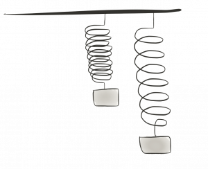
In Newtonian mechanics, the movement of the object is described by the equation

$m \frac{d^2}{dt^2} x=-kx ,$ where $x$ denotes the position of the object and $k$ the spring constant that characterises the mechanical spring. (This is known as Hooke's law.)

The corresponding Hamiltonian, that is used in the Hamiltonian framework to characterise the system is

$H = \frac{1}{2m}p^2 + \frac{k}{2}x^2 \, .$

Starting from this Hamiltonian one can derive the equation of motion $m \frac{d^2}{dt^2} x=-kx$ that is used in the Newtonian framework. The Hamiltonian represents the total energy of the object. This means $H= T+V$ where $T=\frac{1}{2m}p^2$ is the kinetic energy and $V= \frac{k}{2}x^2$ is the potential energy due to the compression and elongation of the spring.

In the Lagrangian framework the same system is characterised by the action

$S = \int dt \left( \frac{m}{2} \left(\frac{dx}{dt}\right) - \frac{k}{2}x^2 \right) ,$ where $L= \frac{m}{2} \left(\frac{dx}{dt}\right) - \frac{k}{2}x^2$ is called the Lagrangian.

Starting from this action, one can derive the equation of motion $m \frac{d^2}{dt^2} x=-kx$ which is used in the Newtonian framework. Moreover, starting from this Lagrangian we can derive the corresponding Hamiltonian through a Legendre transformation. Moreover, we can also derive the Lagrangian from the corresponding Hamiltonian by making use of the Legendre transformation.

To summarize:

Hamiltonian:

\frac{1}{2m}p^2 + \frac{k}{2}x^2

Lagrangian:

\int dt \left( \frac{m}{2} \left(\frac{dx}{dt}\right) - \frac{k}{2}x^2 \right)

Newtonian:

m \frac{d^2}{dt^2} x = -kx

Table adapted from Principles of Quantum Mechanics by R. Shankar ↩

Formalisms

Table of Contents

The Formalisms in Practice

A concrete example