Why is it interesting?

Gauge fields like the photon field or gluon fields are usually described using gauge potentials. An alternative is to use Wilson lines. In contrast to gauge potentials, Wilson loops are completely gauge invariant. The set of all Wilson loops is sufficient to reconstruct the corresponding gauge potential.

The formulation of Yang-Mills theory which makes use of Wilson loops is called loop formulation.

Layman

A particular nice system to understand Wilson loops in a non-technical context are financial markets.

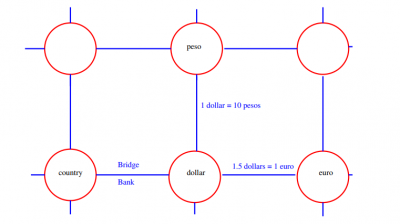
Source: The symmetry and simplicity of the laws of physics and the Higgs boson by Juan Maldacena

Say, we represent different countries by different points on a lattice. Each country has its own currency. However, the absolute values of the different currencies has no meaning of all on the global money market. Instead, all that counts are the relationships between the different currencies. The exchange rates between different currencies is encoded in something we call connection.

Now, how can we make money on the money market?

Well, let's say we are a banker in London. We have a budget of 100 pounds. Our goal is to trade our currency against other currencies in such a way that we have in the end more than 100 pounds. This means, we need to look for profitable loops through the global money lattice. We are interested in loops, because to actually determine if have earned money, we need to compare our final amount of money with the 100 pounds we started with. This is only possible if the final amount of money is also given in pounds.

Let's say the exchange rates are as follows:

• 1.5 dollars = 1 pound,
• 1 dollar = 10 pesos,
• 1 pound = 10 pesos.

How can we make money in this situation?

1. We start by trading our 100 pound against 150 dollars.
2. Then, we trade the 150 dollars against 1500 pesos.
3. Finally we trade the 1500 pesos against 150 pounds.

Thus, by trading in a loop we have gained 50 pounds.

The loops we considered here are exactly analogous to the Wilson loops used in quantum field theories. The gauge freedom corresponds here to the freedom to rescale the local currencies. For examples, England could introduce a new currency called "new-pound" and determine that 1 new-pound is worth 10 pounds. This wouldn't change the situation at the global money market at all, because all banks would simply adjust their exchange rates:

• 0.15 dollars = 1 new-pound,
• 1 dollar = 10 pesos,
• 1 new-pound = 1 pesos.

Absolute value has no meaning and this is what we call gauge freedom. We can't make more money simply because we change the local value of our currency.

The thing we used in the situation above to earn money is called arbitrage. An arbitrage means a possibility to earn money without any risk. The arbitrage possibilities are completely encoded in closed loops.

In physics we usually don't use Wilson loops, but instead work with gauge field strengths (think electric or magnetic field strength). These gauge field strengths $F_{\mu\nu}$ correspond to infinitesimal Wilson loops around a given point $x$.

For more on this perspective see

• Physics of Finance by Kirill Ilinski
• The symmetry and simplicity of the laws of physics and the Higgs boson by Juan Maldacena
• Foreign exchange market as a lattice gauge theory by K. Young

The confining phase is usually defined by the behavior of the action of the Wilson loop, which is simply the path in spacetime traced out by a quark–antiquark pair created at one point and annihilated at another point. In a non-confining theory, the action of such a loop is proportional to its perimeter. However, in a confining theory, the action of the loop is instead proportional to its area. Since the area is proportional to the separation of the quark–antiquark pair, free quarks are suppressed. Mesons are allowed in such a picture, since a loop containing another loop with the opposite orientation has only a small area between the two loops. https://en.wikipedia.org/wiki/Color_confinement

Student

Researcher

Examples

Example1

Example2:

FAQ

History