Intuitive

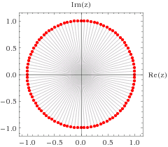
Phase factors $e^{i \theta(\vec x,t)}$, like they appear in quantum mechanics, are just complex numbers with amplitude $1$. Therefore, we can picture them as points on a circle with radius $1$:

The wave function that describes an electron has a specific phase $\Psi(\vec x,t)= |\Psi(\vec x,t)|e^{i \theta(\vec x,t)}$ at each point $\vec x$ at any given moment $t$. Each such phase $\theta$ can be represented by a dot on the unit circle.

Therefore, as an electron moves through space, we have above each point that it passes a specific point on the unit circle that denotes the specific phase that the electron wave function has at this location. A set of unit circles above each space point is like a notebook that keeps track of the phase of the electron at this location.

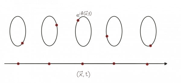
It is convenient to cut the circles such that they become lines. We only need to remember that the end points of these lines need to be identified.

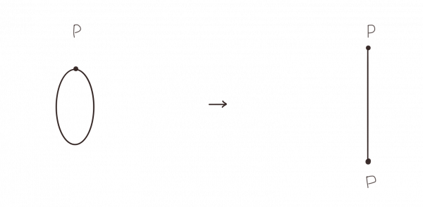
The picture that then emerges, is that we have a line above each point in space. A dot in each such line represents the specific phase our electron has.

In other words, we now have a bundle of circles above the space in which our electron moves. This is an important tool since it allows us nicely to think about how phase factors evolve as a particle moves through space. It is especially useful, as soon as we are dealing with more than one electron.

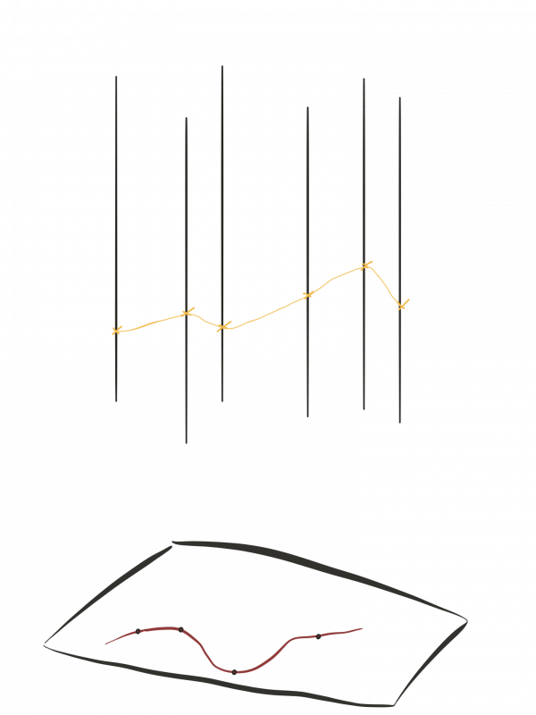
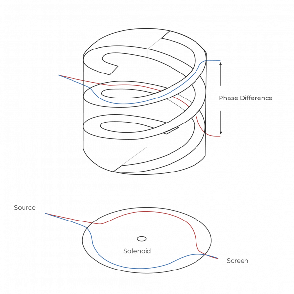
In the lower part of the image we have the actual space where our electron moves. In the upper part of the image we have the "internal" space, which is our fiber bundle. As the particles follows a path in our actual space, it also traces out a path on the fiber bundle.

The actual tool that tells us which path in the fiber bundle our electron will follow is called the connection, and in physics corresponds to the gauge field. We can think of this connection like a family of ramps. Our electron starts at one specific location with one specific phase. Then, as it moves through space the ramps tell us how the phase changes, i.e. which path in the bundle electron traces out:

Now imagine two electrons that follow different path through space, for example, like they do in the Double Slit Experiment or the Aharonov-Bohm experiment. Depending on the physical situation, it can happen that a different path through space also leads to a different path through the fiber. As a result we get a phase difference between the two electrons that is measurable in terms of an interference pattern.

• The best intuitive introduction to fiber bundles is "Fiber Bundles and Quantum Theory" by Herbert J. Bernstein and Anthony V. Phillips. (Can be found for free at Google.)

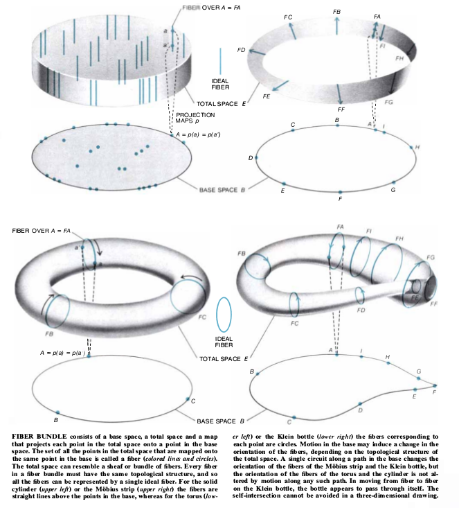
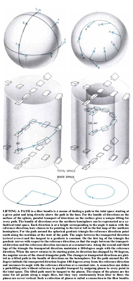
Source: Fiber Bundles and Quantum Theory by Bernstein and Phillips

Concrete

• A nice introduction to fiber bundles with many pictures is Gauge Theories and Fiber Bundles: Definitions, Pictures, and Results by Adam Marsh
• A good textbook on the topic is Topology, Geometry, and Gauge Fields: Foundations by Naber
• For a quick overview with many pictures, see http://gregnaber.com/wp-content/uploads/FIBER-BUNDLES-IN-MATHEMATICS-AND-PHYSICS.pdf

Bundles in Field Theory

A field configuration on a given spacetime Σ is meant to be some kind of quantity assigned to each point of spacetime (each event), such that this assignment varies smoothly with spacetime points. For instance an electromagnetic field configuration is at each point of spacetime a collection of vectors that encode the direction in which a charged particle passing through that point will feel a force (the Lorentz force). This is readily formalized: If

$$ F \in SmthMfd $$ is the smooth manifold of "values" that the the given kind of field may take at any spacetime point, then a field configuration $\Phi$ is modeled as a smooth function from spacetime to this space of values:

$$ \Phi \;\colon\; \Sigma \longrightarrow F \,. $$ It will be useful to unify spacetime and the space of field values into a single space, the Cartesian product

$$ E \; = : \; \Sigma \times F $$ and to think of this equipped with the projection map onto the first factor as a fiber bundle of spaces of field values over spacetime

[…]

This is then called the field bundle, which specifies the kind of values that the given field species may take at any point of spacetime. Since the space $F$ of field values is the fiber of this fiber bundle, it is sometimes also called the field fiber.https://ncatlab.org/nlab/show/field+%28physics%29#AFirstIdeaOfQuantumFields

Abstract

Gravitation, Gauge Theories and Differential Geometry by Tohru Eguchi et. al.

Why is it interesting?

All of physics has two aspects: a local or even infinitesimal aspect, and a global aspect. Much of the standard lore deals just with the local and infinitesimal aspects – the perturbative aspects_ and fiber bundles play little role there. But they are the all-important structure that govern the global – the non-perturbative – aspect. Bundles are the global structure of physical fields and they are irrelevant only for the crude local and perturbative description of reality.

For instance the gauge fields in Yang-Mills theory, hence in EM, in QED and in QCD, hence in the standard model of the known universe, are not really just the local 1-forms $A^a_μ$ known from so many textbooks, but are globally really connections on principal bundles (or their associated bundles) and this is all-important once one passes to non-perturbative Yang-Mills theory, hence to the full story, instead of its infinitesimal or local approximation.https://physics.stackexchange.com/a/77412/37286

Fiber bundles are the appropriate mathematical tool to describe, for example, the physics around a magnetic monopole or also instanton effects. (This is described very nicely in chapter 1 of Topology, Geometry and Gauge fields - Part 1 Foundations by G. Naber). Moreover, non-local aspects like Gribov ambiguities can be understood much more clearly with fiber bundles.

They are also useful to show the similarity between general relativity and Yang-Mills theory, which we use in the standard model. The reformulation of the notions that we usually use in quantum field theory, like the notion of a quantum field, in the fibre bundle formalism, allows us to understand them geometrically. This makes them, contrary to what one may think at the beginning, much less abstract and lets us view at them from a completely new perspective.

See also: https://physics.stackexchange.com/questions/77368/intuitively-why-are-bundles-so-important-in-physics

Although gauge theory is introduced in the above inductive manner for historical and pedagogical reasons it is clear that the essential ingredients -the gauge potential, the gauge field, and the covariant derivative - have an intrinsic mathematical structure which is independent of the context.This structure has been well studied by mathematicians, in the context of differential geometry. In this context transformations g(x) are identified as sections of principal bundles, with Minkowski space J (as base and the Lie groups G as fibres, the scalar and fermion fields are identified as sections of vector bundles with base Jl, the gauge potential as a connection form for G{x), and i^„(x) as the components of the curvature. A review of these aspects is given by Daniel and Viallet (1980). The fibre-bundle formulation is not necessary for dealing with those aspects of gauge theory which are local in M, but it becomes important for understanding problems, such as the axial anomaly (next section) and the gauge-fixing ambiguity (Gribov, 1977; Singer, 1978) which are of global origin. It also shows that gauge theory, and thus the theory of strong, weak and electromagnetic interactions, is basically a geometrical theory. This is not only aesthetically pleasing but brings the unification of weak,electromagnetic and strong interactions with gravitation a step closer. Group Structure of Gauge Theories by Lochlainn O’Raifeartaigh

History

• VECTOR BUNDLES AND CONNECTIONS IN PHYSICS AND MATHEMATICS: SOME HISTORICAL REMARKS by V. S. Varadarajan