
Lagrange Multiplier
Prerequisites: Calculus.
Intuitive
- More people should know about Lagrange multipliers by Brian Skinner
Sometimes you want to maximize something (profit, health, utility, floor space) but subject to a constraint. A Lagrange multiplier is an extra variable introduced for each constraint. At the maximum it tells you how much the maximum value would change if the constraint were loosened a little.
Concrete
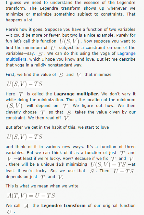
https://johncarlosbaez.wordpress.com/2012/01/19/classical-mechanics-versus-thermodynamics-part-1/
- No-Nonsense Classical Mechanics by Jakob Schwichtenberg, appendix "Lagrange Multipliers"
Abstract
Let be a smooth manifold, smooth, and smooth with a regular value. Then is an embedded submanifold of codimension with tangent spaces . A point is a critical point of exactly when vanishes on . A linear functional vanishes on the common kernel of if and only if it is a linear combination of them, so the condition is
for unique numbers (unique because the are linearly independent). Equivalently, is an unconstrained critical point of the Lagrange function on . Geometrically, lies in the conormal space of at . Whether a critical point is a maximum or minimum is decided by the Hessian of in at fixed , restricted to .
Multipliers as sensitivities. Replace the constraint by and let be the value of at a nondegenerate constrained extremum that depends smoothly on . Then
This is how multipliers acquire physical meaning. Maximizing the entropy subject to and gives , where is the multiplier of the energy constraint. The sensitivity formula gives , so temperature enters as a Lagrange multiplier. In mechanics with holonomic constraints , the equations of motion are , and is the constraint force.
Duality. For the problem of minimizing subject to , the dual function is a lower bound on the constrained minimum for every (weak duality). For convex problems that satisfy a constraint qualification such as Slater's condition, the largest of these bounds equals the constrained minimum (strong duality). Inequality constraints lead to the Karush-Kuhn-Tucker conditions, with sign-constrained multipliers that vanish for inactive constraints. In thermodynamics the switch from the constrained problem (fixed ) to the unconstrained one (fixed ) is a Legendre transformation: with the distribution above, , so that is the free energy.