Intuitive

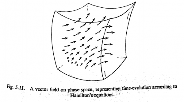
Now, how are we to visualize Hamilton's equations in terms of phase space? First, we should bear in mind what a single point Q of phase space actually represents. It corresponds to a particular set of values for all the position coordinates $x_1,x_2,\ldots.$ and for all the momentum coordinates $p_1,p_2, … $ That is to say, Q represents our entire physical system, with a particular state of motion specified for every single one of its constituent particles. Hamilton's equations tell us what the rates of change of all these coordinates are when we know their present values; i.e. it governs how all the individual particles are to move. Translated into phase-space language, the equations are telling us how a single point Q in phase space must move, given the present location of Q in phase space. Thus, at each point of phase space, we have a little arrow - more correctly a vector- which tells us the way that Q is moving, in order to describe the evolution of our entire system in time. The whole arrangement of arrows constitutes what is known as a vector field (Fig. .11). Hamilton's equations thus define a vector field on phase space.

Let us see how physical determinism is to be interpreted in tel filS of phase space. For initial data at time t = 0, we would have a particular set of values ~specified for all the position and momentum coordinates; that is to say, we have a particular choice of point Q in phase space. To find the evolution of the system in time. we simply follow the arrows. Thus the entire evolution of our system with time - no matter how complicated that system might be - is described in phase space as just a single point moving along following the particular arrows that it encounters. We can think of the arrows as indicating the "velocity" of our point Q in phase space. For a "long" arrow, Q moves along swiftly, but if the arrow is "short", Q's motion will be sluggish. To see what our physical system is doing at time t, we simply look to see where Q has moved to, by that time, by following arrows in this way. Clearly, this is a deterministic procedure. The way that Q moves is completely determined by, the Hamiltonian vector field.

page 174ff in "The Emperors new Mind" by R. Penrose

Concrete

Hamiltons equations are $$ \dot q = \frac{\partial H}{\partial p} \\ \dot p = - \frac{\partial H}{\partial q} $$

These equations tell you how to move a point in phase space infinitesimally given a scalar function H on the phase space. Such a transformation is an infinitesimal canonical transformation.

Time evolution of an Observable

In general, the time derivative of a function $F$ that is a function of generalized position and momentum coordinates, but not a direct function of time (which is often accurate) is

$$\frac{dF}{dt}=\frac{\partial F}{\partial q}\frac{dq}{dt}+\frac{\partial F}{\partial p}\frac{dp}{dt}$$

Using Hamilton's equation we get

$$ \frac{dF}{dt}=\frac{\partial F}{\partial q}\frac{\partial H}{\partial p}-\frac{\partial F}{\partial p}\frac{\partial H}{\partial q}\equiv \{H,F\},$$

where $\{H,F\}$ denotes the Poisson bracket. Take note that there is a close connection between this equation and the Heisenberg equation in quantum mechanics: $$\frac{\mathrm{d}\hat F}{\mathrm{d}t} = -\frac{i}{\hbar}[\hat F,\hat H] + \frac{\partial \hat F}{\partial t}.$$

Abstract

If a first order ODE can be written in the form $$ \dot s = \mathbb J \frac{\partial H}{\partial s} $$

where $\mathcal S$ is a $2n$ dimensional manifold, and $\mathbb J$ a $2n\times 2n$ symplectic matrix of the form $$ \mathbb J = \left( \begin{matrix} 0 & \mathbb{I}_{n\times n} \\ -\mathbb{I}_{n\times n} & 0 \end{matrix}\right) $$ for some function $H:\mathcal S \to \mathbb R$, it is said that the equations form a Hamiltoinian System with Hamiltonian Funciton $H$.

Why is it interesting?

Hamilton's Equations are a way of rewriting Newton's Second Law of Motion on a first-order system of differential equations, i.e, it only has first derivatives in time.

This comes at the cost of doubling the size of the system.