Intuitive

In Lagrangian mechanics we derive how a particle will evolve using the idea that ‘total amount that happened’ from one moment to another as a particle traces out a path is minimal.

So formulated differently, the basic idea is that nature is lazy. All we have to do is find the laziest way to realize something and this is exactly how nature will behave.

Concrete

In Lagrangian mechanics we define a quantity \begin{equation} L\equiv K(t)-V(q(t)) \end{equation} called the Lagrangian. In addition, for any trajectory $q$ with $q(t_0)=a$, $q(t_1)=b$, we we define the corresponding action \begin{equation} S(q)\equiv \int_{t_0}^{t_1}L(t)\,dt. \end{equation}

The basic idea is now that nature causes particles to follow the trajectories with the least amount of action.

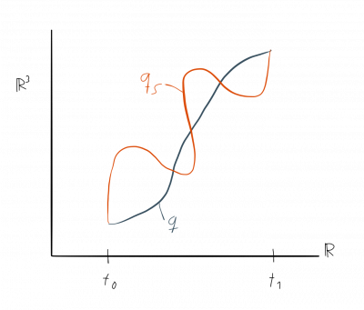
In the image on the right-hand side this could be the solid line denotes by $q$. Another path is shown as a dashed line and denoted by $q(s)$.

The Lagrangian approach assigns to each path a quantity called action as defined above and then tells us that the correct path that an object really follows is the path with minimal action. In our example the path $q$ could have an action of $3$ and the path $q_s$ an action of $5$. Hence, path $q$ is correct and not path $q_s$.

The mathematical toolset that we use to find the paths with minima action is known as variational calculus.

The final result using this machinery is that the path with minimal action is the one that satisfies the Euler-Lagrange equations.

Using the Lagrangian approach, we can derive Newtonian mechanics. Alternatively, we can start with Newtonian mechanics and derive Lagrangian mechanics.

Derivation of Newton's second law

A point with minimal action is $S$ defined through the condition \begin{equation} \left. \frac{d}{ds}S(q_s)\right|_{s=0} = 0 \end{equation} where \[ q_s = q + s\delta q \] for all $\delta q \colon [t_0,t_1]\rightarrow\mathbb{R}^n$ with \[ \delta q(t_0)=\delta q(t_1)=0. \] We want to derive \begin{equation} F=ma \quad \Leftrightarrow \quad \left.\frac{d}{ds} S(q_s)\right|_{s=0}=0 \; \textrm{for all} \; \delta q\colon [t_0,t_1]\rightarrow\mathbb{R}^n \; \textrm{with}\; \delta q(t_0)=\delta q(t_1)=0. \end{equation} To do this, we now use the definition of the action and the chain rule: \[ \begin{split} \left.\frac{d}{ds}S(q_s)\right|_{s=0} &= \frac{d}{ds}\left.\int_{t_0}^{t_1} \frac{1}{2}m\dot{q}_s(t)\cdot\dot{q}_s(t)-V(q_s(t))\,dt\right|_{s=0} \\ \\ &= \left.\int_{t_0}^{t_1}\frac{d}{ds}\left[ \frac{1}{2}m\dot{q}_s(t) \cdot \dot{q}_s(t) - V(q_s(t))\right]dt\right|_{s=0} \\ \\ &= \left.\int_{t_0}^{t_1}\left[ m\dot{q}_s \cdot \frac{d}{ds}\dot{q}_s(t)- \nabla V(q_s(t)) \cdot \frac{d}{ds}q_s(t)\right]dt\right|_{s=0} \\ \end{split} \] Next we note that \[ \frac{d}{ds} q_s (t) = \delta q(t) \] so \[ \frac{d}{ds} \dot{q}_s (t) = \frac{d}{ds} \frac{d}{dt} {q}_s (t) = \frac{d}{dt} \frac{d}{ds} {q}_s (t) = \frac{d}{dt} \delta{q}(t) .\] Therefore we have \[ \begin{split} \left.\frac{d}{ds}S(q_s)\right|_{s=0} &= \int_{t_0}^{t_1}\left[ m\dot{q} \cdot \frac{d}{dt} \delta q(t) - \nabla V(q(t)) \cdot \delta q(t)\right]dt . \end{split} \] Finally, we can integrate by parts and note that the boundary terms vanish because $\delta q=0$ at $t_1$ and $t_0$: \[ \begin{split} \frac{d}{ds}S(q_s)\rvert_{s=0} &= \left.\int_{t_0}^{t_1}\left[ -m\ddot{q}(t)-\nabla V(q(t))\right] \cdot \delta q(t) dt\right. . \\ \end{split} \] Looking at this, we can see that the variation of the action vanishes for all possible variations $\delta q$ if and only if the term in brackets is exactly zero: \[ -m\ddot{q}(t)-\nabla V(q(t)) = 0. \] Therefore, the correct path $q$ with a minimal amount of action $S$ is the one that follows from the equation \[ F=ma. \]

Examples

Harmonic Oscillator

The Lagrangian in classical mechanics is given by the kinetic energy $ \cal T$ minus the potential energy $ \cal U$:

$$ \cal L=T-U . $$

Therefore, a harmonic oscillator in the Lagrangian framework is characterized by the action

$$ S = \int dt \left( \frac{m}{2} \left(\frac{dx}{dt}\right) - \frac{k}{2}x^2 \right) ,$$ where $L= \frac{m}{2} \left(\frac{dx}{dt}\right) - \frac{k}{2}x^2$ is the Lagrangian.

Starting from this action, we can derive the equation of motion by using the Euler-Lagrange equation.

$$ \frac{\partial {\cal L}}{\partial x}-\frac{d}{dt}(\frac{\partial {\cal L}}{\partial dot{x}})= 0 $$

$$ \Rightarrow m \frac{d^2}{dt^2} x -kx= 0$$

Pendulum

The Lagrangian for the pendulum can be written \[{\cal L=T-U}=\frac{mr^2\dot{\theta}^2}{2}+mgr\cos\theta\] The equation of motion is \[\frac{\partial {\cal L}}{\partial \theta}-\frac{d}{dt}(\frac{\partial {\cal L}}{\partial dot{\theta}})= -mgr\sin\theta-mr^2\frac{d\dot\theta}{dt}=0\] giving: \[\ddot{\theta}+\frac{g}{r}\sin\theta=0\]

Small Amplitude Approximation

If $\theta <<1$ then $\sin\theta\approx\theta$ and \[\frac{d^2\theta}{dt^2}+\frac{g}{r}\theta\] This solution describes simple harmonic motion \[\theta=A\cos(\omega t-\phi)\] where \[\omega=\sqrt{\frac{g}{r}}\] and the constants $A$ and $\phi$ are determined from the initial condition E.g. if $\theta=0,\;t=0$ then $\phi=\pm \frac{\pi}{2}$. If $d\theta/dt=0,\;t=0$ then $\phi=0,$ or $\pi$ (depending on whether the pendulum is moving to the left or right initially) The period is \[\tau=\frac{2\pi}{\omega}=2\pi\sqrt{\frac{r}{g}}\]

Finite Amplitude

If the amplitude is not small we have to solve the nonlinear equation \[\frac{d^2\theta}{dt^2}+\frac{g}{r}\sin \theta=0\] (nonlinear because sin $\theta$ is a nonlinear function of the dependent variable $\theta$.)

The Atwood Machine

A frictionless pulley with two masses, $m_1$ and $m_2$, hanging from it.

We have \begin{align*} K &= \frac{1}{2}(m_1+m_2)(\frac{d}{dt}(\ell-x))^2 = \frac{1}{2}(m_1+m_2)\dot{x}^2 \\ V &= -m_1 g x - m_2 g(\ell-x) \\ \text{so } L &= K-V = \frac{1}{2}(m_1+m_2)\dot{x}^2 + m_1gx+m_2g(\ell-x) \end{align*} The configuration space is $Q=(0,\ell)$, and $x\in(0,\ell)$. Moreover $TQ=(0,\ell)\times\mathbb{R}\ni(x,\dot{x})$. As usual $L:TQ\rightarrow\mathbb{R}$. Note that solutions of the Euler-Lagrange equations will only be defined for \emph{some} time $t\in\mathbb{R}$, as eventually the solutions reaches the ``edge'' of $Q$.

The momentum is: \[ p = \frac{\partial L}{\partial\dot{x}} = (m_1+m_2)\dot{x} \] and the force is: \[ F = \frac{\partial L}{\partial x} = (m_1-m_2)g \] The Euler-Lagrange equations say \begin{align*} \dot{p} &= F \\ (m_1+m_2)\ddot{x} &= (m_1-m_2)g \\ \ddot{x} &= \frac{m_1-m_2}{m_1+m_2}g \end{align*} So this is like a falling object in a downwards gravitational acceleration $a=\left(\frac{m_1-m_2}{m_1+m_2}\right)g$.

We integrate the expression for $\ddot{x}$ twice to obtain the general solution to the motion $x(t)$. Note that $\ddot{x}=0$ when $m_1=m_2$, and $\ddot{x}=g$ if $m_2=0$.

Reading Recommendations

• The best book on Lagrangian mechanics is The Lazy Universe by Coopersmith
• Many problems with solutions are collected in Schaum's Outline of Theory and Problems of Theoretical Mechanics by Murray R Spiegel

Abstract

Lagrangian mechanics can be formulated geometrically using fibre bundles.

The Lagrangian function is defined on the tangent bundle $T(C)$ of the configuration space $C$.

In contrast, the Hamiltonian function is defined on the cotangent bundle $T^\star(C)$, which is also called phase space.

The map from $T^\star(C) \leftrightarrow T(C)$ is called Legendre transformation.

• Lectures on Mechanics by Marsden
• See page 471 in Road to Reality by R. Penrose, page 167 in Geometric Methods of Mathematical Physics by B. Schutz and http://philsci-archive.pitt.edu/2362/1/Part1ButterfForBub.pdf.

Why is it interesting?