Why is it interesting?

The Sine-Gordon model is a toy model that helps to understand fundamental notions like duality in a simplified setup.

In addition, the equations of the theory permit topological non-trivial solutions called solitons. Many basic features of such solitons can be studied in the Sine-Gordon model in a simplified setup.

The name "Sine-Gordon model" is a wordplay, because the equation of motion of the model is similar to the famous Klein-Gordon equation and contains a sinus function.

Layman

Student

Specification of the Model

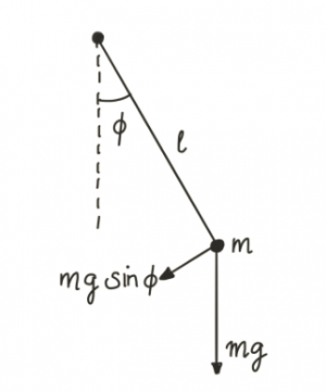
The Sine-Gordon model describes a continuous set of pendulums. Each pendulum hangs freely in a uniform gravitational field of strength $g$ on a rod with length $l$. The excitation above the ground state is measured by the angle $\phi$. At the end of the pendulum, we have a bob of mass $m$. This is shown in the picture on the right-hand side.

The Lagrangian of the system is

$$ L = \frac{1}{2} ml^2\dot{\phi}^2 - mgl (1-cos \phi), $$ where $\dot{\phi}\equiv d\phi /dt $ denotes the time derivative.

To analyze the system it is convenient to rescale the units such that all constants $m,g,l$ are equal to one. Then, the Lagrangian reads

$$ L = \frac{1}{2} \dot{\phi}^2 - (1-cos \phi). $$

So far, this could be a normal mechanics problem. However, if $\phi$ becomes not only a variable that depends on $\phi = \phi(t)$, but also on the location $\phi(t,x)$ we have a continuous set of such pendulums and hence are dealing with a field theory.

We assume that we have an infinite set of such pendulums that hang from an also infinitely long support rod.

The thing is now that neighboring pendulums are coupled to each other. This could be achieved, for example, through elastic bands between the pendulums.

In a field theory, we are not interested in the Lagrangian but in the Lagrangian density since we are interested in what happens locally. The Lagrangian density for the Sine-Gordon field theory reads

$$ \mathscr{L} = \frac{1}{2} \left( (\partial_\mu \phi)^2 \right) - (1-cos \phi), $$ $$ = \frac{1}{2} \left( \dot{\phi}^2 - (\partial_x \phi)^2 \right) - (1-cos \phi).$$ where $ L = \int_{-\infty}^\infty dx\mathscr{L} $ and $\mu =0,1$.

Now that we have the Lagrangian density, we can derive the equations of motion of the system, as usual, by using the Euler-Lagrange equations

$$\frac{\partial \mathscr{L}}{\partial \Phi^i} - \partial_\mu \left(\frac{\partial \mathscr{L}}{\partial(\partial_\mu\Phi^i)}\right) = 0$$

which yields

$$ \partial_\mu \partial^\mu \phi + \sing \phi =0\, . $$

When we now want to understand what the system actually does, we must search for solutions of this field equation. Before doing that, we want to think about what kind of solutions we can except.

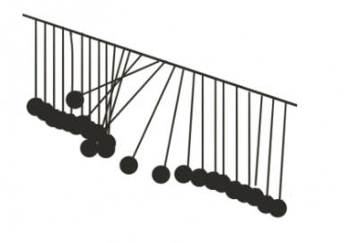
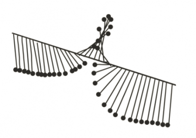
Most importantly, since the pendulums are coupled it possible that waves travel through the set of pendulums. Think of a "laola wave" that travels through a sports stadium.

In addition, to such normal waves, we can also have solitary waves that travel through the system. Imagine we pick one end of the support rod and rotate it by $360^\circ$. This will yield a twist in the system and as a result, a solitary wave will travel through the system.

This is shown in the image on the right-hand side.

The ground state of the system is when all pendulums are hanging straight down.

Recommended Resources:

• https://www.uni-muenster.de/Physik.TP/archive/fileadmin/lehre/NumMethoden/WS0910/ScriptPDE/SineGordon.pdf

Researcher

Examples

Example1

Example2:

FAQ

History

The Sine-Gordon equation was originally used to study surfaces of constant negative curvature in geometry: E. Bour, J. Ecole Imperiale Polytech. 19, 1 (1862)