Add a new page:
Add a new page:
This is an old revision of the document!
The Scalar 1+1 Model describes how the simplest type of field interacts with itself.
The simplest type of field is a field with no internal angular momentum and called scalar field.
In addition, the model is a model in only one space dimension plus the usual time dimension. (That's what the 1+1 in the name of the model means). This is the simplest setup where we can investigate dynamics.
The physics described by the Scalar 1+1 Model model looks like this:
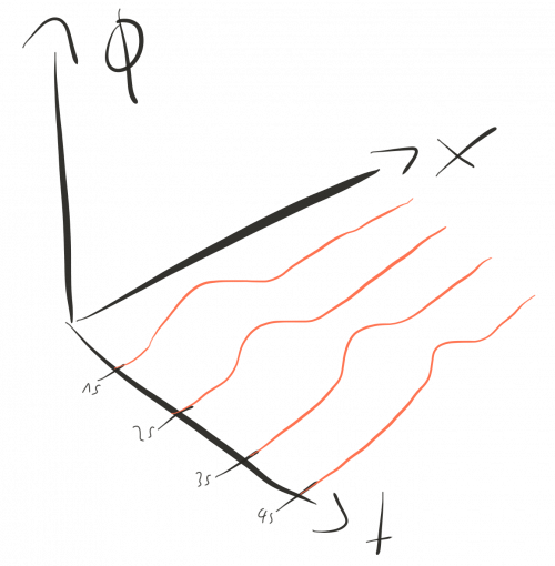
Each red line shows a field configuration at a given point in time.

The model only contains a real scalar field $\phi (x) \in \mathbb{R}$. The scalar potential is
$$ U= \frac{\lambda}{2} ( \phi^2-a^2)^2, $$
and is conveniently normalized such that the ground state (the vacuum solution) is at $U=0$. In addition, the potential is bounded from below $U\geq 0$.
The field equation is
$$ \partial_{x_i}^2 \phi = 2 \lambda \phi (\phi^2-a^2). $$
It is important to note that this field equation is a non-linear differential equation and hence allows non-linear solutions.
The field equation can be either derived from the action of the model or from the energy functional:
$$ E= \int dx^2 \left[ \frac{1}{2} \left( \frac{\partial \phi}{\partial \vec x}\right)^2 + U(\phi)\right]. $$
Then, demanding that the variation $\delta E$ vanishes yields the field equation.
Standard Solutions
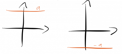
The standard solutions of the field equation are simply
$$ \phi_c = \pm a. $$
These two solutions are the classical vacuum solution. They are rather boring since the field simply takes the vacuum value, either $a$ or $-a$ everywhere.
Solitonic Solutions - The Kink
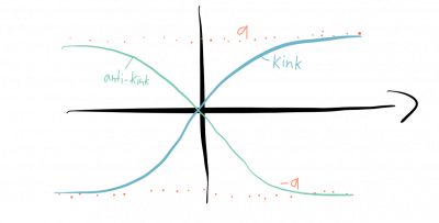
In addition, we can find other less trivial solutions:
$$ \phi_k^\pm = \pm a \tanh(\sqrt{\lambda} ax_i) .$$
These solutions are called the kink and the anti-kink solution. It is important to note that these solutions are time-independent. In this sense they are non-dissipative, i.e. do not vanish over time like normal wave solutions do.
We can check that $\phi_k^\pm $ is a solution by putting it into the field equations.
On the left-hand side of the field equation we get if we put $\phi_k^+$ in:
\begin{align} \partial_{x_i}^2 \tilde{\phi_k^+} &= \partial_{x_i}^2 \tanh(\sqrt{\tilde{\lambda}} x_i) \\ & = - 2 \tilde{\lambda} \frac{\sinh}{\cosh^3}.\end{align}
On the right-hand side, ignoring all constants and only focussing on the functions, we get
\begin{align} \tilde{\phi_k^+} ((\phi_k^+)^2-1) &\propto \tanh (\tanh^2-1) \\ &= \tanh \left(\frac{\sinh^2}{\cosh^2}-1\right) \\ &= \tanh \left(\frac{\sinh^2}{\cosh^2}-\frac{\cosh^2}{\cosh^2}\right) \\ &= \tanh \left(\frac{\sinh^2-\cosh^2}{\cosh^2}\right) \\ &= \tanh \frac{1}{\cosh^2} \\ &= \frac{\sinh}{\cosh} \frac{1}{\cosh^2} \\ &= \frac{\sinh}{\cosh^3} .\\ \end{align}
Thus, the right-hand side and the left-hand side of field equations yield exactly the same when we put $\phi_k^+$ in and therefore these functions really solve the field equations.
Properties of the Kink Solution
We are interested in finite energy solution since infinite energy solutions would require infinite energy to create.
To make sure that our kink solution has finite energy we need the boundary conditions that the scalar field only takes ground state values at infinity, i.e. either $a$ or $-a$. The ground state has zero energy and hence this requirement basically just means that we demand that the field energy vanishes at infinity.
We can write these boundary conditions mathematically:
$$ \phi(\infty) - \phi(-\infty) \stackrel{!}{=} 2na, $$ where $n \in (0,-1,+1)$.
These boundary conditions become important when we discover that there is a conserved current in the model:
$$ j_\mu (x) = \epsilon_{\mu \nu} \partial^\nu \phi(x), $$ where $\epsilon_{\mu \nu} $ is the two-dimensional Levi-Civita symbol. This current is conserved since partial derivatives commute and $\epsilon_{\mu \nu}$ is totally antisymmetric. A sum over something symmetric $\partial \mu \partial^\nu$ times something totally antisymmetric $\epsilon_{\mu \nu}$ yields zero:
$$ \partial^\mu j_\mu (x) = 0. $$
Whenever we have conserved current, we can find a conserved charge:
\begin{align}Q &= \int_{-\infty}^\infty dx j_0 \notag \\ & = \int_{-\infty}^\infty dx ( \epsilon_{0 0} \partial^0 \phi(x) + \epsilon_{0 1} \partial^1 \phi(x) ) \\ & = \int_{-\infty}^\infty dx \partial^1 \phi(x) \\ & = \int_{-\infty}^\infty dx \partial^x \phi(x) \\ &= \phi(\infty) - \phi(-\infty) = 2na \, . \end{align}
The conserved quantity is, therefore, $n$, up to a constant factor. This conserved quantity is known as winding number of the kink and because of this topological conserved quantity, the kink is stable.
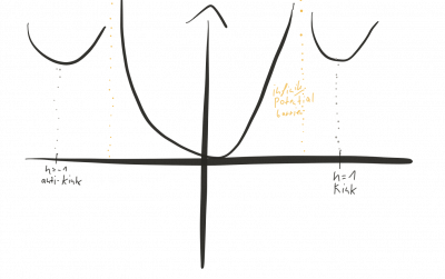
We can understand the stability of the kink also by looking at the energy density of the various solutions. Between the kink and the standard vacuum solution, there is an infinite potential barrier. This barrier exists since it would take an infinite amount of energy to change the kink solution to a classical energy solution. The kink solutions would need to be transformed at every spacetime point either to $a$ or to $-a$ and since the space we are considering is infinite, this transformation would take an infinite amount of energy.
The spacetime we are considering is $1+1$ dimensional. Hence the boundary of space is just two points $x_-=-\infty$ and $x_+ =\infty$. We denote this boundary of space with $S_\infty = \{ -\infty, \infty \}$.
The scalar field $\phi$ takes at infinity only vacuum values since otherwise, we would be dealing with an infinite energy configuration. The vacuum manifold is also just two points: $M_V = \{ -a, a \}$.
Our restriction to solutions with finite energy means implies that we are dealing with maps $ S_\infty \to M_V $, i.e. at infinity the field only takes values in the vacuum manifold.
Now, topology tells us that such maps can be classified through an integer $n$. This number then automatically labels our solitonic solutions.
The scalar model in one spatial and one temporal dimension is the simplest type of model we can construct in field theory.
It is often used to introduce the basics of solitonic solutions, since the Scalar 1+1 model contains a non-trivial kink solution.
