Intuitive

A gauge model is a model where the way different particles or fields interact with each other is determined by a gauge symmetry.

The particles that mediate the gauge interaction are called gauge bosons.

Gauge theory means we use abstract symmetries, called $U(1)$, $SU(2)$ and $SU(3)$ to derive the correct terms in the Lagrangian that describe interactions.

Concrete

The basic idea behind gauge theories is that the fundamental symmetries of nature actually dictate the interactions between the fields of nature.

Mathematically Yang-Mills theory is described by the Yang-Mills equation.

If the gauge symmetry is abelian the Yang-Mills equation reduces to the Maxwell equations.

Here is the idea behind gauge theories in a nutshell:

Consider a field $\Psi$ representing electrically charged matter. The free field obeys the Dirac equation which is just the Euler–Lagrange equation(s) for the Lagrangian (density) $L_{Dirac} = \bar \Psi(i\gamma^\mu ∂μ - m)\Psi$.The corresponding action is clearly invariant under so-called ‘global’ U (1) phase transformations: $\Psi \to e^{iq\Lambda} \Psi$, $\bar \Psi \to e^{-iq\Lambda} \bar \Psi$ with $\Lambda$ a constant. It follows from Noether’s first theorem that when the equations of motion are satisfied there will be a corresponding conserved current.

Consider now ‘localizing’ these phase transformations, i.e. letting $\Lambda$ become an arbitrary function of the coordinates $\Lambda(x):$ $\Psi \to e^{iq\Lambda(x)} \Psi$, $\bar \Psi \to e^{-iq\Lambda(x)} \bar \Psi$. As it stands, the free field Lagrangian is clearly not invariant under such transformations, since the derivatives of the arbitrary functions, i.e. $∂μ \Lambda(x)$, will not vanish in general. The Lagrangian must be modified if the theory is to admit the local transformations as (variational) symmetries. In particular, we replace the free field Lagrangian with $$L_{interacting} = \bar \Psi(i\gamma^\mu ∂μ - m)\Psi - q A_μ \bar \Psi γ^\mu \Psi ≡ L_{Dirac} - J_μ A^μ ,$$ with $J_μ = q \bar \Psi \gamma_\mu \Psi$. This current is in fact the conserved current associated with the global U(1) invariance of the interacting theory. Towards securing local invariance we have introduced the field $A_μ$, the gauge potential. The particular form of coupling between the matter field and this gauge potential in $L_{interacting}$ is termed minimal coupling.

This modified Lagrangian is now invariant under the local phase transformations provided that the vector field $A_μ$ is simultaneously transformed according to $A_μ (x) → A_μ(x) - ∂_μ \Lambda(x)$. electromagnetic potential.

“On continuous symmetries and the foundations of modern physics” by CHRISTOPHER A. MARTIN

The Lagrangian that we derive by demanding local invariance describes perfectly quantum electrodynamics. More specifically, this means the new term $- q A_μ \bar \Psi γ^\mu \Psi$ in the Lagrangian, that we wrote down to ensure local invariance, is exactly the correct term to describe, for example, how an electron interactions with a photon.

One often hears physicists say "to gauge a symmetry group." It means to localize the group or to make the transformation parameters vary spatiotemporally so that the system does not behave as a unit under the transformations. Local transformations allow a large degree of individuality for each point of a system by endowing it with an autonomous internal structure.The Poincare transformations become local in general relativity. The quantum phase transformation is localized and becomes exp[iO(x)] in quantum field theories. Local symmetries are ubiquitous in quantum field theories. The symmetry groups U(l), SU(2) x C/(7), and SU(3) for the electromagnetic, electro-weak, and strong interactions are all local transformations whose parameters are functions of spatiotemporal positions. These local symmetry groups are often called gauge groups and theories employing them gauge field theories.They determine the properties of the phase space at each spatiotemporal point individually. A local symmetry is more complicated than a global symmetry because it demands the global invariance of the entire system under local transformations. Generally, this requires the introduction of extra structures to reconcile the difference of various local transformations. The extra structures are usually interpreted as interaction potentials, as discussed in the next chapter. From "How is Quantum Field Theory possible" by Auyang

In general, the Lagrangian in a gauge theory reads

\begin{equation} \mathcal{L}=-\frac 12 Tr (F_{\mu\nu}F^{\mu\nu})\\ =-\frac 14 F_a^{\mu\nu}F^a_{\mu\nu} \end{equation}

where \begin{equation} F^{\mu\nu}=F_a^{\mu\nu}t_a \end{equation} and $t_a$ are the generators of the Lie group satisfying \begin{equation} Tr(t_at_b)=\frac 12 \delta_{ab} \quad [t_b,t_c]=i f_{abc}t_a \end{equation} The structure constants $f_{abc}=f^{abc}$ are selected antisymmetric in all indices. The gauge field \begin{equation} A^{\mu}=A_a^{\mu}t_a \end{equation} defines the curvature $F^{\mu\nu}$ by \begin{equation} F^{\mu\nu}=\partial^{\mu}A^{\nu}-\partial^{\nu}A^{\mu}+ig[A^{\mu},A^{\nu}]\\ \end{equation} In component form this gives \begin{equation} F^{\mu\nu}_a=\partial^{\mu}A_a^{\nu}-\partial^{\nu}A_a^{\mu}-gf_{abc}A^{\mu}_bA^{\nu}_c \end{equation}

Curvature is antisymmetric \begin{equation} F^{\mu\nu}=-F^{\nu\mu} \end{equation} The number $g$ is called coupling constant, and \begin{equation} \partial^{\mu}=\frac {\partial}{\partial x_{\mu}} \quad \partial_{\mu}=\frac {\partial}{\partial x^{\mu}} \end{equation} are partial derivatives with respect to the contravariant coordinates $x^{\mu}$ and contravariant coordinates $x_{\mu}=g_{\mu\nu}x^{\nu}$. $x^0=ct$ and $x^j$, $1\le j\le 3$, are the space coordinates.

Recommended Textbooks:

• Gauge Theories in Particle Physics by Aitchison, Hey
• A good introduction can be found here http://www.damtp.cam.ac.uk/user/ch558/pdf/Gauge_theories.pdf
• Also great: http://isites.harvard.edu/fs/docs/icb.topic1146666.files/IV-1-YangMills.pdf
• Quarks, Leptons and Gauge fields by Huang.

An extremely popular book is "Gauge Theory of elementary particle physics" by Cheng and Li. However, take note that it is quite dense and thus hard for beginners to understand. However, once you understand what gauge theories are all about, this book is nice to look things up.

Abstract

• A great introduction to the geometric perspective on gauge theories can be found in “Geometrical methods of mathematical physics” by Bernard F. Schutz at page 219
• See also Quantum Yang-Mills Theory by Jaffe and Witten
• Another great introduction to the fibre bundle formulation of gauge theories with many nice pictures is Gauge Theories and Fiber Bundles: Definitions, Pictures, and Results by Adam Marsh
• A pedagogical introduction to the loop formulation of gauge theory can be found in the book Some Elementary Gauge Theory Concepts by Sheung Tsun Tsou, Hong-Mo Chan.

Recommended Resources:

• For a great high-level introduction to Yang-Mills theory, see Topology, Geometry and Gauge Fields: Foundations by Naber and also the second part Topology, Geometry and Gauge Fields: Interactions.
• Atiyah M. Geometry of Yang-Mills Fields
• Baez, J. and Muniain, J. P.: Gauge Fields, Knots and Gravity. World Scientific Publishing Co Inc, 1994. and especially, the nice summary by Michael Nielsen.
• http://www.damtp.cam.ac.uk/user/dbs26/AQFT/YM.pdf
• The geometrical setting of gauge theories of the Yang-Mills type by M. Daniel and C. M. Viallet

See also

• What is a gauge? by Terence Tao
• Quantum Field Theory: A Modern Perspective by V. Parameswaran Nair
• Geometry and topology of chiral anomalies in gauge theories by R. Rennie
• Gravitation, Gauge Theories and Differential Geometry by Tohru Eguchi et. al.
• Why gauge Symmetry by J. Gegelia

Geometry of Gauge Theories

Source: Concept of nonintegrable phase factors and global formulation of gauge fields by Tai Tsun Wu and Chen Ning Yang

Source

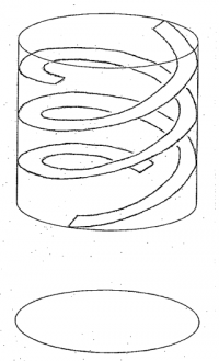
Mathematically, the gauge symmetry means that we a copy of the gauge group above each spacetime point. Each continuous symmetry is at the same time also a manifold. The collection of all these symmetries is called a fiber bundle.

The gauge fields are Ehresmann connections on the bundle, i.e. objects that tell us how we have to move in the bundle when we move through spacetime. Intuitively we can think of the connections as ramps that tells us how the phase of a field changes as it moves through space

The field strength corresponds to the curvature of the fiber bundle.

Gauge theory in terms of differential forms

Instead of the the traditional Lagrangian, we can also write the action of a gauge theory using the four-form \begin{equation} \mathcal{A}=Tr F\wedge *F=F_{\mu\nu}^aF_{\mu\nu}^a d^4x \end{equation} and the action is then \begin{equation} \mathcal{S}=\frac {1}{4g^2}\int \mathcal{A} \end{equation}

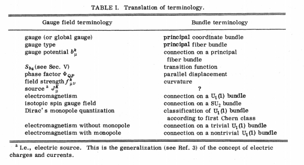
Although gauge theory is introduced in the above inductive manner for historical and pedagogical reasons it is clear that the essential ingredients -the gauge potential, the gauge field, and the covariant derivative - have an intrinsic mathematical structure which is independent of the context.This structure has been well studied by mathematicians, in the context of differential geometry. In this context transformations g(x) are identified as sections of principal bundles, with Minkowski space J (as base and the Lie groups G as fibres, the scalar and fermion fields are identified as sections of vector bundles with base Jl, the gauge potential as a connection form for G{x), and i^„(x) as the components of the curvature. A review of these aspects is given by Daniel and Viallet (1980). The fibre-bundle formulation is not necessary for dealing with those aspects of gauge theory which are local in M, but it becomes important for understanding problems, such as the axial anomaly (next section) and the gauge-fixing ambiguity (Gribov, 1977; Singer, 1978) which are of global origin. It also shows that gauge theory, and thus the theory of strong, weak and electromagnetic interactions, is basically a geometrical theory. This is not only aesthetically pleasing but brings the unification of weak,electromagnetic and strong interactions with gravitation a step closer. Group Structure of Gauge Theories by Lochlainn O’Raifeartaigh

Incidentally, for physicists, essentially all bundles are trivial and trivialized. Then they write coordinate-full formulas for the transition maps, especially when doing gauge theory. As mathematicians, we know that there are lots of bundles that are not trivializable, although every bundle is locally so. To a physicist, when a bundle is not trivializable, they call it an "anomaly. So anyway, to describe a bundle to a physicist, you only need to describe the fiber. To describe a particle, you need to give a bundle and an action, and this data should be gauge and Poincare invariant.

http://mathoverflow.net/questions/16507/spins-as-tensor-fields/16510#16510

Why is it interesting?

The best theories of nature that we have

• Quantum Electrodynamics
• Quantum Chromodynamics
• The Standard Model

are gauge theories.

Physical theories of fundamental significance tend to be gauge theories. These are theories in which the physical system being dealt with is described by more variables than there are physically independent degree of freedom. The physically meaningful degrees of freedom then reemerge as being those invariant under a transformation connecting the variables (gauge transformation). Thus, one introduces extra variables to make the description more transparent and brings in at the same time a gauge symmetry to extract the physically relevant content. It is a remarkable occurrence that the road to progress has invariably been towards enlarging the number of variables and introducing a more powerful symmetry rather than conversely aiming at reducing the number of variables and eliminating the symmetry Henneaux M. & Teitelboim C., Quantization of gauge systems, Princeton University Press, Princeton, 1992.

Gauge theories are interesting because they are the most general class of renormalizable field theories, and we certainly need a field theory to be renormalizable if it is to function calculably all the way from $m_p ~ 10^{19}$ GeV down to atomic mass scales.Fermion masses and Higgs representations in SU(5) by John Ellis and Mary K. Gaillard

History

For a nice discussion of the history of gauge theories, see "Gauge Fields" by Robert Mills.

FAQ

How can we describe physical particles in a gauge theory?

A question not often addressed when discussing the standard model is how one describes physical particles. Taking the electron as an example, the assumption usually made is that the free Dirac spinor in the interacting theory, at asymptotic times, can be viewed as an electron since ‘the coupling switches off’. This would mean that what is being caught in a detector is really a free fermion. The problem here, of course, is that in QED and QCD the coupling does not switch off, and assuming it does so generates infrared divergences. As a result, the spinors do not become free even at asymptotic times [1, 2], nor do they ever become gauge invariant. […]

The physical picture is of a matter particle surrounded by a cloud of ‘photons’, neither of which are individually observable, but which together constitute a gauge invariant, physical particle. This description is nonlocal, which is an immediate consequence of gauge invariance, but observables calculated with our states are manifestly local and correctly reproduce classically expected physics.

Stability, creation and annihilation of charges in gauge theories by Anton Ilderton, Martin Lavelle, David McMullan

Take note that the physical spectrum can be quite different from what we would expect naively by using gauge dependent spinors etc. In the standard model it is somewhat of a miracle that the naive approach yields the same as the approach that uses gauge invariant quantities. However, in theories beyond the standard model the spectrum can turn out to be quite different. See, for example, this nice discussion and the references therein.

What makes Yang-Mills theories so difficult to work with?

The hardest problem in Yang-Mills theory is the problem of reduction of the gauge symmetry (redundancy); i.e. the characterization of the orbit space of gauge potentials modulo gauge transformations.

In 3+1 dimensions, this space is awfully complicated both geometrically and topologically. The solution of this problem should shed light to the longstanding open problems in Yang-Mills theory such as the mass gap and confinement. The reduced orbit space is infinite dimensional and not even a manifold.

If we knew a solution of this problem, we could, in principle, quantize the reduced configuration space (by means of geometric quantization, which is itself a formidable problem) and obtain the quantum Yang-Mills which should reflect the above conjectured properties.

Most of the known methods (except lattice regularization) use gauge fixing (together with Feddeev-Popov ghosts and BRST) to reduce the gauge redundancy. This method reduces the gauge redundancy only approximately as it suffers from the problem of Gribov copies. It is believed that this approximation is valid only in perturbation theory. There are several non-perturbative approximations such as the Faddeev-Niemi theory, but their connection to Yang-Mills is only heuristic.

Two physicists: Gurd Rudolf and Matthias Schmidt (together with a number of collaborators) are working on several methods to tackle this hard problem by reducing the gauge redundancy without gauge fixing. They have many publications on the subject. They use mainly methods of geometry and topology. Their efforts led to certain classification results of the yang-Mills gauge orbit. They wrote a book named Differential geometry and Mathematical physics (Part 1 , Part 2).

In the book, they give a detailed account of the basics of geometry and topology relevant to the Yang-Mills theory in a rigorous mathematical presentation. The entire book can be viewed, however, as an introduction to the last two chapters of Part 2 where they give account of some of their results in the classification and quantization of the Yang-Mills theory. This subject is very hard. Their research is still ongoing. They have results for certain toy models, such as a lattice of a single plaquette. They tackle both problems of the classical characterization of the orbit space and its quantization for these models. The book covers many advanced topics and can be a useful reference for a physicist interested in Yang-Mills theory research, and quantization.https://physics.stackexchange.com/a/368458/37286

Research

“The gauge principle is generally regarded as the most fundamental cornerstone of modern theoretical physics. In my view its elucidation is the most pressing problem in current philosophy of physics.”Michael Redhead